Quarto is a file type used to create technical reports while including both R code, or other programming languages, and output in a document. A qmd1 file is a fancy R Script containing extra capabilities. Additionally, qmd files allow for citations, footnotes, mathematical expressions, links, and much more. Once the document is finished, it can be rendered to a word file, pdf, html file, and much more. Quarto is the considered the next generation of RMarkdown.
25.2 Anatomy of a Quarto Document
There are three main components in an qmd file: the YAML header, R code, and basic text.
The YAML header contains information on how to render the document. It is located at the beginning of the document surrounded by 3 dashes (---) above and below it. For starters, the YAML header will contain a ‘title’, ‘author’, ‘date’, and ‘output’ line.
The R code is located in a block known as chunks. A chunk tells RStudio to read the next lines as code. A chunk begins with three back ticks followed by {r} and ends with three back ticks. Everything in between the back ticks will be executed by R. In RStudio, a chunk can be inserted using the keyboard shortcut ctrl+alt+I or cmd+option+I.
An example of an R chunk is shown below:
```{r}mean(mtcars$mpg)```
The R chunk will be rendered as below:
mean(mtcars$mpg)
Notice the chunk includes the code in a block followed by the output from the console.
The last component of an qmd document is the text. Write anywhere in the document, and it will be rendered as is.
25.3 Chunk Options
R chunks have options that will alter how the code or the output is rendered. The chunk options can be set either globally to affect the entire qmd document or locally to affect only an individual chunk. For more information about chunk options, visit https://yihui.org/knitr/options/
25.3.1 Global Chunk Options
To set global chunks options, add the two lines to YAML header:
---knitr: opts_chunk: ---
Followed by the chunks and R options you want to set:
A couple of recommended chunk options set globally are eval: false, and tidy: styler. These options make rendering the document easier.
One chunk option is tidy: styler. This tells Quarto to prevent code from printing in a long line, possibly off the page. For example, look at the output of this chunk:
## This comment is designed to show what happens when all your code is in 1 line. This is fine when you are coding, but when you are putting it in a report, it will run off the page.
Notice the comment being printed off the page. Using the options tidy: styler, the chunk is rendered as
## This comment is designed to show what happens when all## your code is in 1 line. This is fine when you are## coding, but when you are putting it in a report, it will## run off the page.
The last 2 lines control how R will compute and print output. R.Options: tells Quarto that the options R will be changed, and each line after alters options. digits: 2 indicates R to use 2 significant digits.
25.3.2 Local Chunk Options
Local chunk options can be used to control an individual chunk will behave. To control a specific chunk, place the option below the {r} identifier and use the #| chunk option indicator. An example is povided below:
The chunk option eval set to false tells Quarto to not evaluate the code within the chunk. Notice how the output was not printed the R chunk above. When we set eval to true, the output is printed:
```{r}#| eval: truemean(mtcars$mpg)```
[1] 20.1
The echo option will control if the code within the chunk should be printed in the document. This next chunk contains #| echo: true:
mean(mtcars$mpg)
[1] 20.1
Now the chunk contains #| echo: false:
[1] 20.1
The R Code disappears.
There are chunk options for figures as well. A few options are fig-height, fig-width, fig-align, and fig-cap.
This chunk contains fig-height: 3.5; fig-width: 3.5; fig-align: left.
The chunk options tells RStudio to create an image that is 3.5 inches in height and width, and align the image to the left.
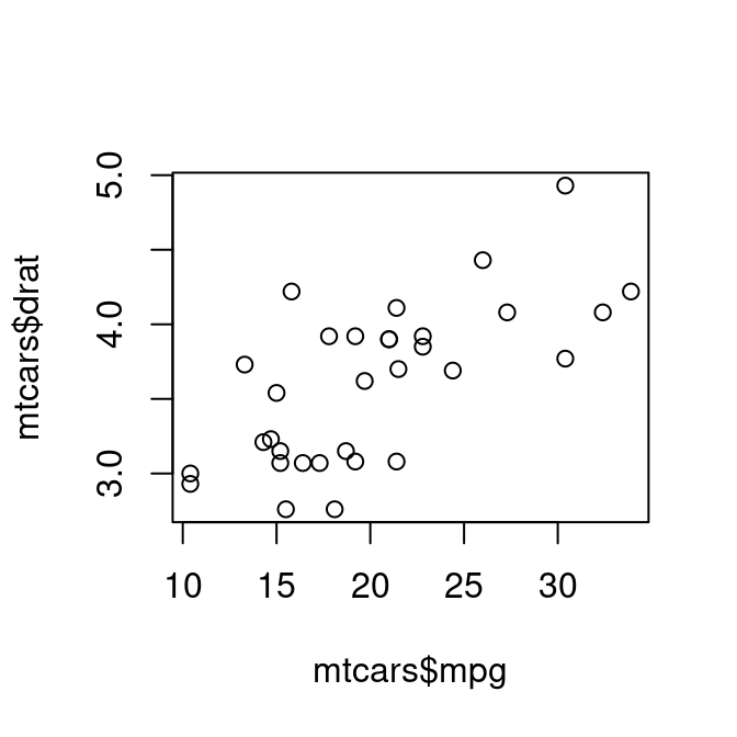
The following chunk contains fig-height: 3.5; fig-width: 3.5; fig-align: left; fig-cap: "This is a scatter plot of MTCARS' MPG and DRAT"; label: fig-mtcars.
```{r}#| eval: true#| fig-height: 3.5#| fig-width: 3.5#| fig-align: center#| fig-cap: "This is a scatter plot of MTCARS' MPG and DRAT"#| label: fig-mtcarsplot(mtcars$mpg, mtcars$drat)```
Figure 25.1: This is a scatter plot of MTCARS’ MPG and DRAT
The chunk adds a caption with fig-cap and reference label with label. The label of the plot can be referenced later in the document. Figure 25.1 can be referenced with @fig-mtcars.
25.3.3 Inline Code
Instead of evaluating code in a chunk, code can evaluated in the text instead. For example, if we want to write the mean mpg in mtcars is 20.090625, one can type {r} mean(mtcars$mpg), surrounded by back ticks (`), instead of writing the entire number and risk of miscopying the results.
25.4 Formatting
Qmd files contain basic formatting capabilities. The use of the # followed by text creates a heading. Using two or more # symbols will create subheadings based on the number of #. A text is italicized by surrounding the text with one asterisk (*italicized*). A text is boldfaced by surrounding it with 2 asterisk (**boldfaced**).
To create an unordered list, use the - symbol at the beginning of each line. To create a sub-item, press the tab button twice (4 spaces), then the - symbol. Repeat this method for further sub-items.
First Item
Second Item
First Sub-Item
First Sub-Sub-Item
First Sub-Sub-Sub-Item
To created an ordered list, type the number followed by a period for each line. To create sub-lists, press the tab button twice and order them appropriately.
First
Second
First
Second
First
Second
A block quote is created with the > symbol at the beginning of a line.
Qmd files allows a table to be constructed in 2 ways, manually or using a package such as the gt package. A table is manually created by using |, :, and -. The first line contains | and the column names in between. The second line contains |:-|:-| which indicates how the table is aligned. The location of : symbol just tells RStudio about the alignment. Below is the example code of Table 25.3:
The last line will adds a caption to the table and {#tbl-greektable} creates a label to reference the table in the text using @tbl-greektable.
The gt function from the gt package creates a table from a data frame or R object. Here is an example code to create a table from the first 6 rows of the mtcars dataset:
Notice that Table 25.1 is easily produced using the gt() function with a caption
Table Table 25.1 is referenced by using the label created in the chunk and the @tbl-mtcarsdata. To install gt run the following line in your console:
install.packages("gt")
25.5 Citations and Referneces
Qmd documents contains capabilities to add citations and a bibliography. For example, to cite this textbook (Mendenhall and Sincich 2012), use the @ symbol followed by a citation identifier from the .bib file surrounded by square brackets, [@mendenhallSecondCourseStatistics2012]. To cite your textbook again (2012) without the authors names, use a - sign in front of the @ symbol, [-@mendenhallSecondCourseStatistics2012]. To cite multiple books (Casella and Berger 1990; Rohatgi and Saleh 2015; Resnick 2014; Erich L. Lehmann and Casella 1998; E. L. Lehmann and Romano 2005), add each citation inside the square brackets with the @ symbol and separate them with semicolons, [@casellaStatisticalInference1990; @rohatgiIntroductionProbabilityStatistics2015; @resnickProbabilityPath2014; @lehmannTheoryPointEstimation1998; @lehmannTestingStatisticalHypotheses2005].
The references will be added automatically at the end of the document.
In order to use citations and references, the qmd file needs needs a .bib file containing all the information of the references. First, save the .bib file in the same folder (directory) as your qmd file. Then add the line bibliography: NAME.bib to the YAML header. Make any changes appropriately to the line, such as the name of the .bib file.
25.5.1.bib File
The .bib file is an ordinary text file containing “bib” entries with information about each reference. Below is an example bib entry about R:
@Manual{,
  title = {R: A Language and Environment for Statistical Computing},
  author = {{R Core Team}},
  organization = {R Foundation for Statistical Computing},
  address = {Vienna, Austria},
  year = {2023},
  url = {https://www.R-project.org/},
}
Creating a .bib file is tedious; however, there are reference managers that can help. I recommend using Zotero, an open-source reference manager designed to import and manage citations. Once a citation is in Zotero, you can export your library as a .bib file. Make sure to check your references in Zotero for any mistakes.
25.6 Math
Quarto is capable of writing mathematical formulas using LaTeX code. A mathematical symbol can be written inline using single $ signs. For example, $\alpha$ is viewed as \(\alpha\) in a document. To write mathematical formulas on its own line use $$. For example, $$Y=mX+b$$ is viewed as \[Y=mX+b\].
25.6.1 Mathematical Notation
Table 25.2: LaTeX syntax for common examples.
Notation
code
\(x=y\)
$x=y$
\(x>y\)
$x>y$
\(x<y\)
$x<y$
\(x\geq y\)
$x\geq y$
\(x\leq y\)
$x\leq y$
\(x^{y}\)
$x^{y}$
\(x_{y}\)
$x_{y}$
\(\bar x\)
$\bar x$
\(\hat x\)
$\hat x$
\(\tilde x\)
$\tilde x$
\(\frac{x}{y}\)
$\frac{x}{y}$
\(\frac{\partial x}{\partial y}\)
$\frac{\partial x}{\partial y}$
\(x\in A\)
$x\in A$
\(x\subset A\)
$x\subset A$
\(x\subseteq A\)
$x\subseteq A$
\(x\cup A\)
$x\cup A$
\(x\cap A\)
$x\cap A$
\(\{1,2,3\}\)
$\{1,2,3\}$
\(\int_a^bf(x)dx\)
$\int_a^bf(x)dx$
\(\left\{\int_a^bf(x)dx\right\}\)
$\left\{\int_a^bf(x)dx\right\}$
\(\sum^n_{i=1}x_i\)
$\sum^n_{i=1}x_i$
\(\prod^n_{i=1}x_i\)
$\prod^n_{i=1}x_i$
\(\lim_{x\to0}f(x)\)
$\lim_{x\to0}f(x)$
\(X\sim \Gamma(\alpha,\beta)\)
$X\sim \Gamma(\alpha,\beta)$
25.6.2 Greek Letters
Table 25.3: LaTeX syntax for greek letters.
Letter
Lowercase
Code
Uppercase
Code
alpha
\(\alpha\)
\alpha
–
–
beta
\(\beta\)
\beta
–
–
gamma
\(\gamma\)
\gamma
\(\Gamma\)
\Gamma
delta
\(\delta\)
\delta
\(\Delta\)
\Delta
epsilon
\(\epsilon\)
\epsilon
–
–
zeta
\(\zeta\)
\zeta
–
–
eta
\(\eta\)
\eta
–
–
theta
\(\theta\)
\theta
\(\Theta\)
\Theta
iota
\(\iota\)
\iota
–
–
kappa
\(\kappa\)
\kappa
–
–
lambda
\(\lambda\)
\lambda
\(\Lambda\)
\Lambda
mu
\(\mu\)
\mu
–
–
nu
\(\nu\)
\nu
–
–
xi
\(\xi\)
\xi
\(\Xi\)
\Xi
pi
\(\pi\)
\pi
\(\Pi\)
\pi
rho
\(\rho\)
\rho
–
–
sigma
\(\sigma\)
\sigma
\(\Sigma\)
\Sigma
tau
\(\tau\)
\tau
–
–
upsilon
\(\upsilon\)
\upsilon
\(\Upsilon\)
\Upsilon
phi
\(\phi\)
\phi
\(\Phi\)
\Phi
chi
\(\chi\)
\chi
–
–
psi
\(\psi\)
\psi
\(\Psi\)
\Psi
omega
\(\omega\)
\omega
\(\Omega\)
\Omega
varepsilon
\(\varepsilon\)
\varepsilon
–
–
25.7 Rendering a Document
A qmd file can be rendered into either an html file, pdf document or word document. Rendering the qmd file to an html file or word document can be easily done using the knit button above. However, rendering the qmd file to a pdf document requires LaTeX to be installed. There are two methods to install LaTeX: from the LaTeX website or from R. I recommend installing the full LaTeX distribution from the https://www.latex-project.org/get/. This provides you with everything you may need. You can also install it from R:
Render your document often so it easier to identify problems with rendering
The Visual Mode in RStudio eases the process of creating a document and makes it more bearable.
YAML is tricky with spacing. Make sure that spaces when indenting options. Also make sure that there are not extra spaces at the end of each line.
25.9 References
Casella, George, and Roger L. Berger. 1990. Statistical Inference. The Wadsworth & Brooks/Cole Statistics/Probability Series. Pacific Grove, Calif: Brooks/Cole PubCo.
Lehmann, E. L., and Joseph P. Romano. 2005. Testing Statistical Hypotheses. 3rd ed. Springer Texts in Statistics. New York: Springer.
Lehmann, Erich L., and George Casella. 1998. Theory of Point Estimation. Second Edition. Springer Texts in Statistics. New York, NY: Springer New York.
Mendenhall, William, and Terry Sincich. 2012. A Second Course in Statistics: Regression Analysis. Seventh edition. Boston: Prentice Hall.
Resnick, Sidney I. 2014. A Probability Path. Modern Birkhäuser Classics. New York: Birkhäuser.
Rohatgi, V. K., and A. K. Md Ehsanes Saleh. 2015. An Introduction to Probability and Statistics. Third edition. Wiley Series in Probability and Statistics. Hoboken, New Jersey: Wiley.