               mpg cyl disp  hp drat    wt  qsec vs am gear carb
Mazda RX4     21.0   6  160 110 3.90 2.620 16.46  0  1    4    4
Mazda RX4 Wag 21.0   6  160 110 3.90 2.875 17.02  0  1    4    4
Datsun 710 22.8 4 108 93 3.85 2.320 18.61 1 1 4 1Data Processing
UC Riverside
4/21/2022
Base Plot
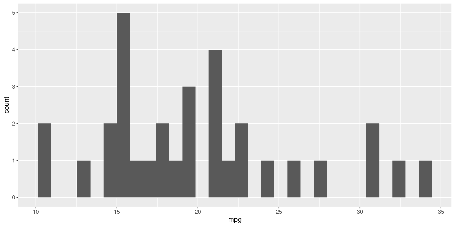
Histograms
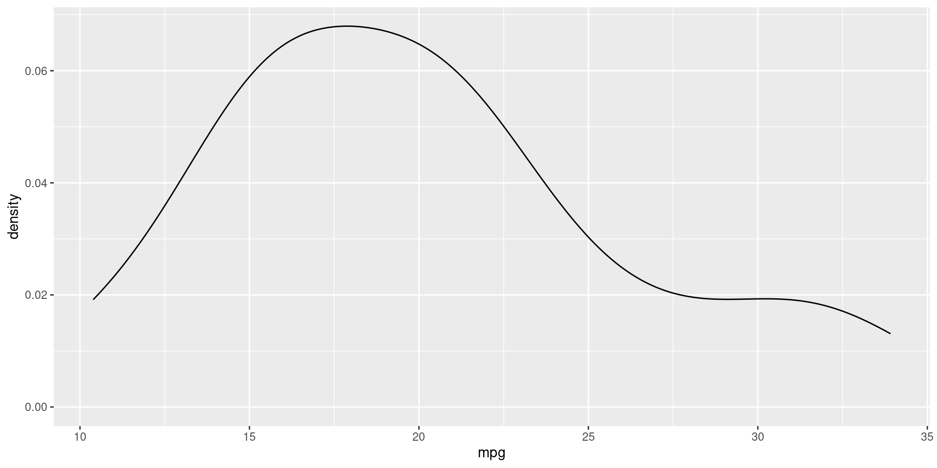
Density Plot
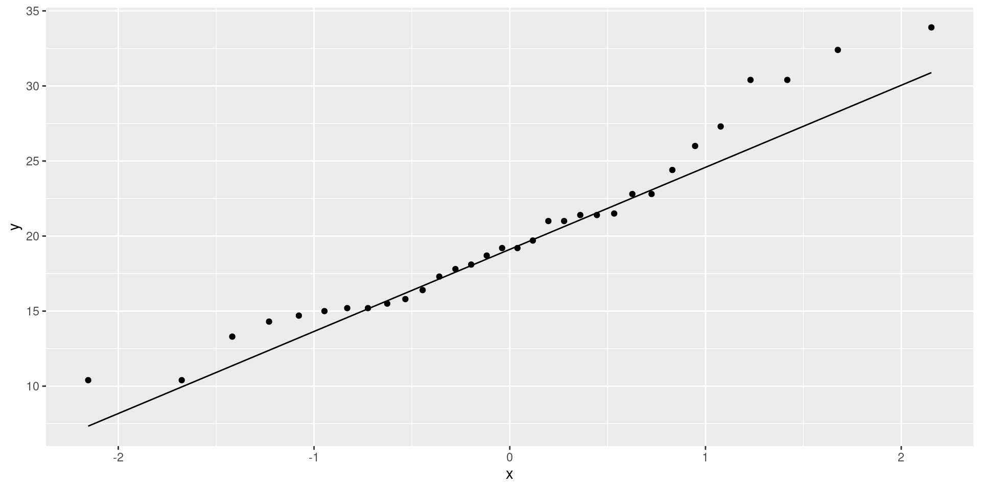
QQ Plot
Bivariate Base Plot
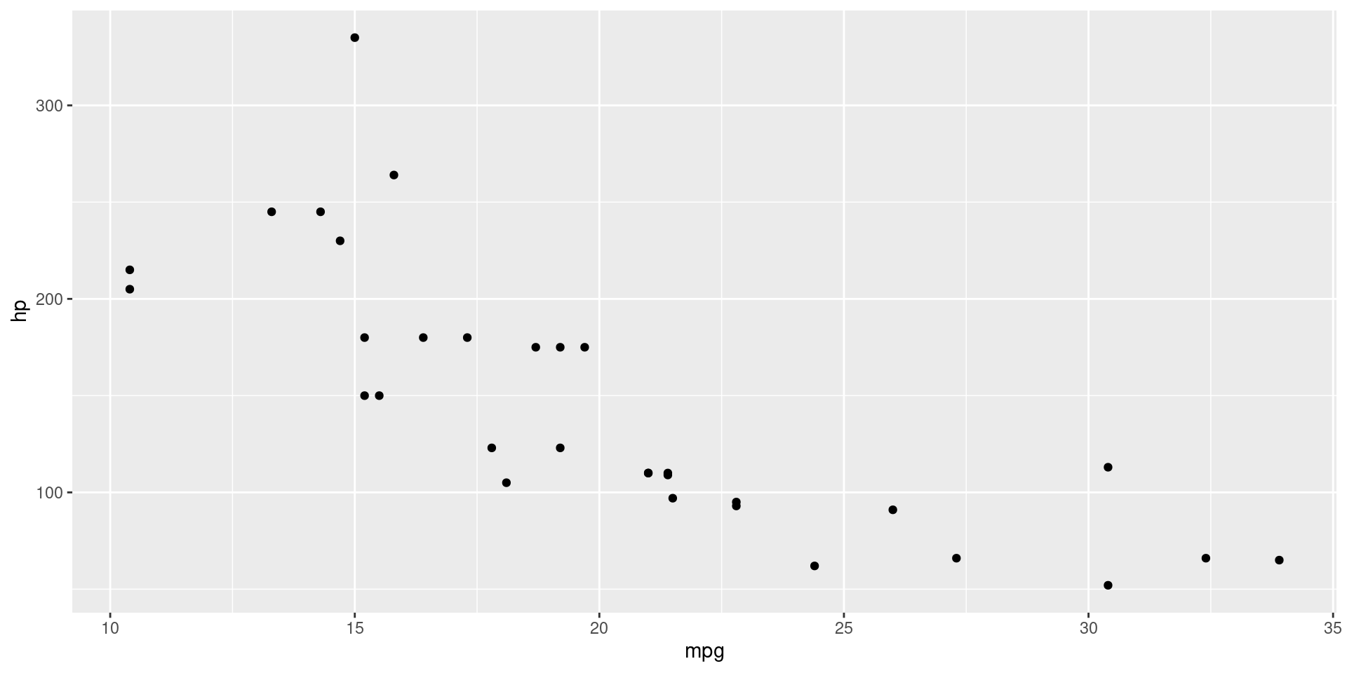
Scatter Plot
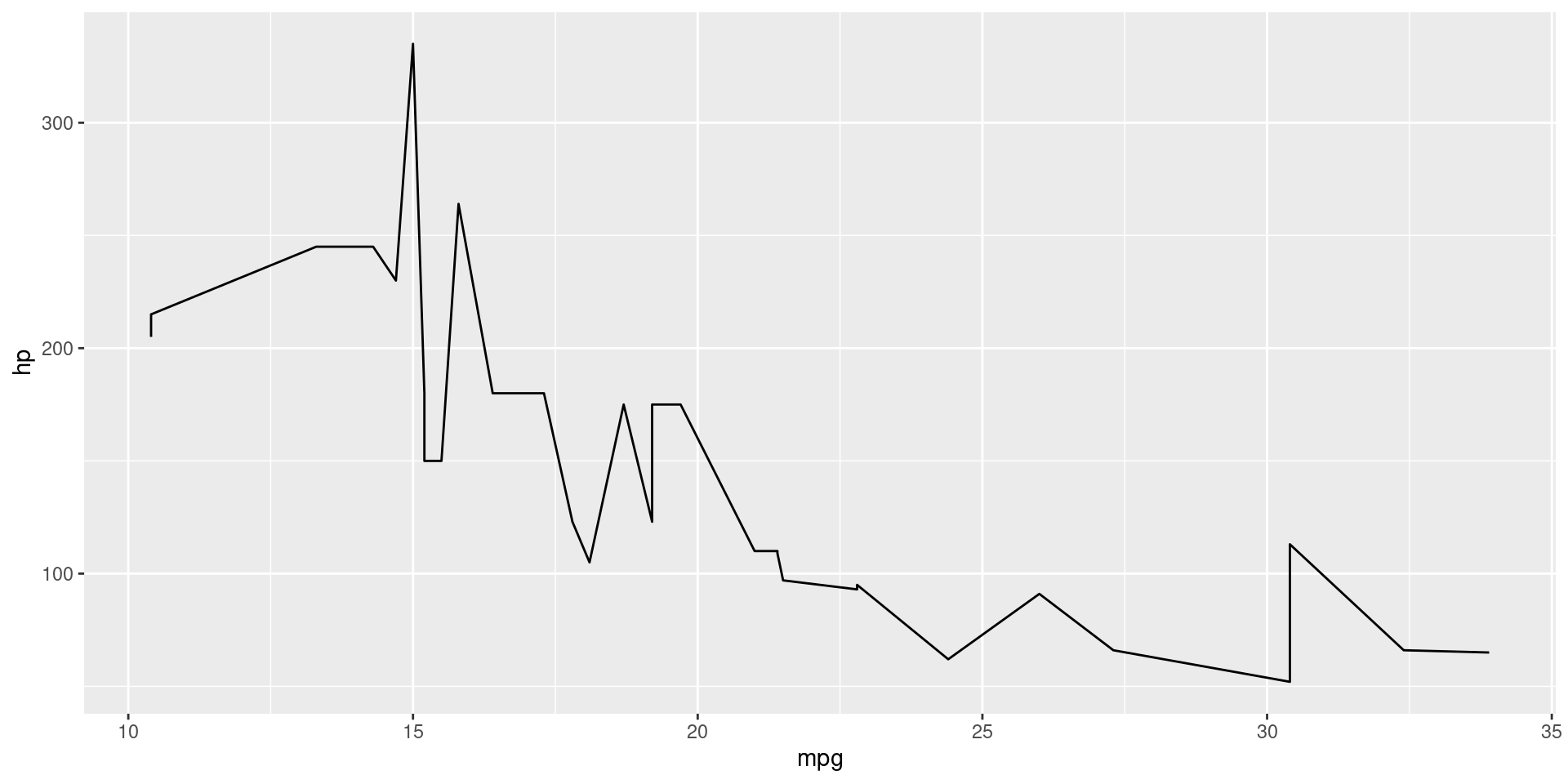
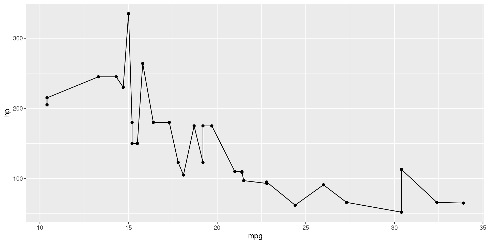
Line Plot
Line & Scatter Plot
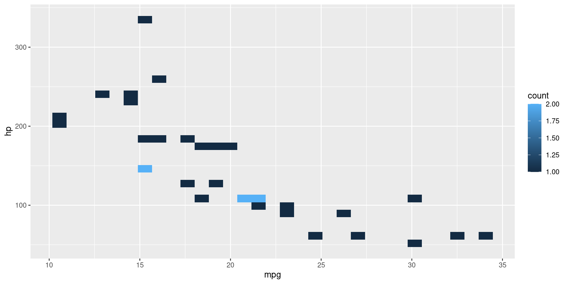
Heat Map
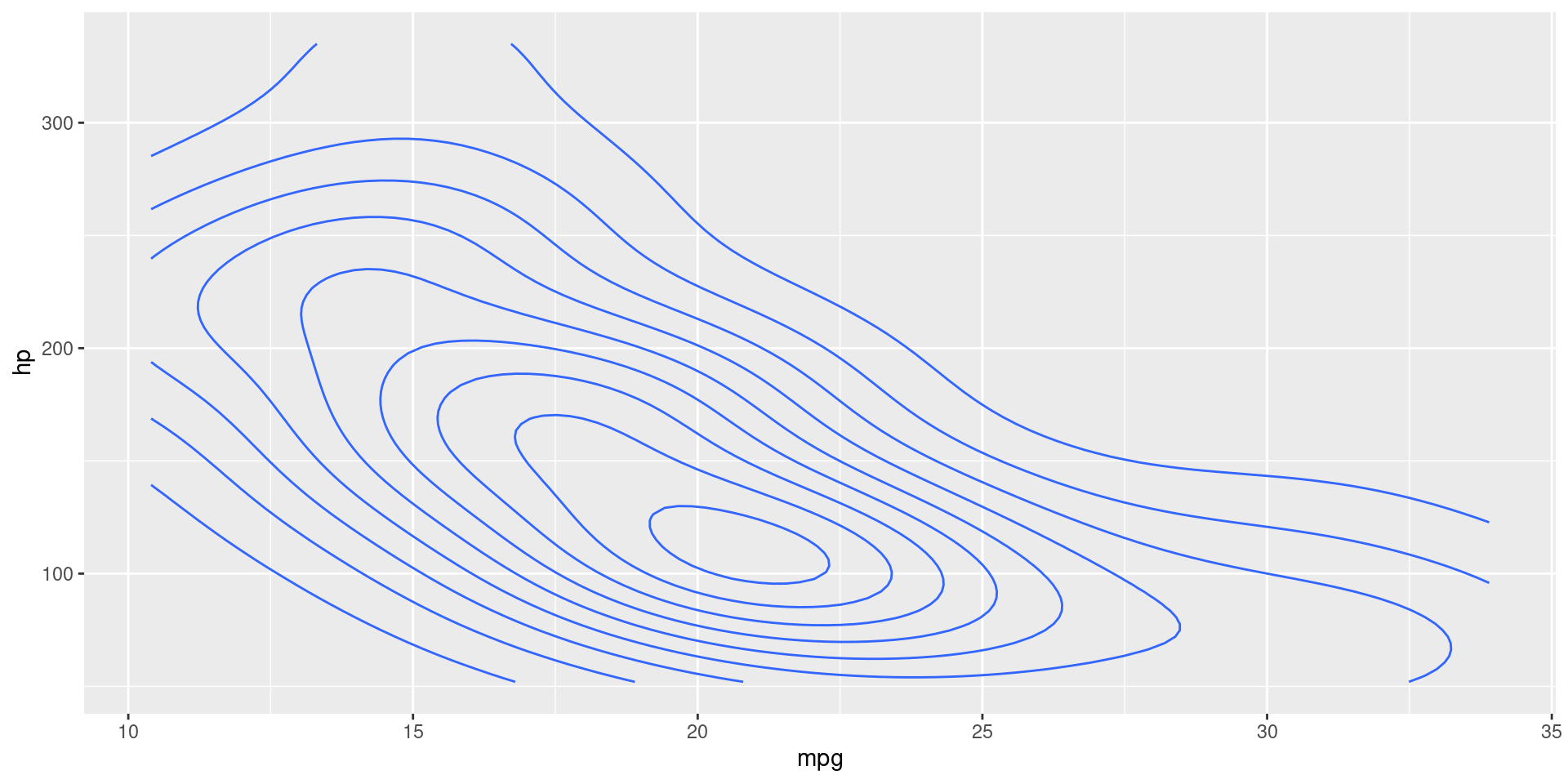
Contour Map
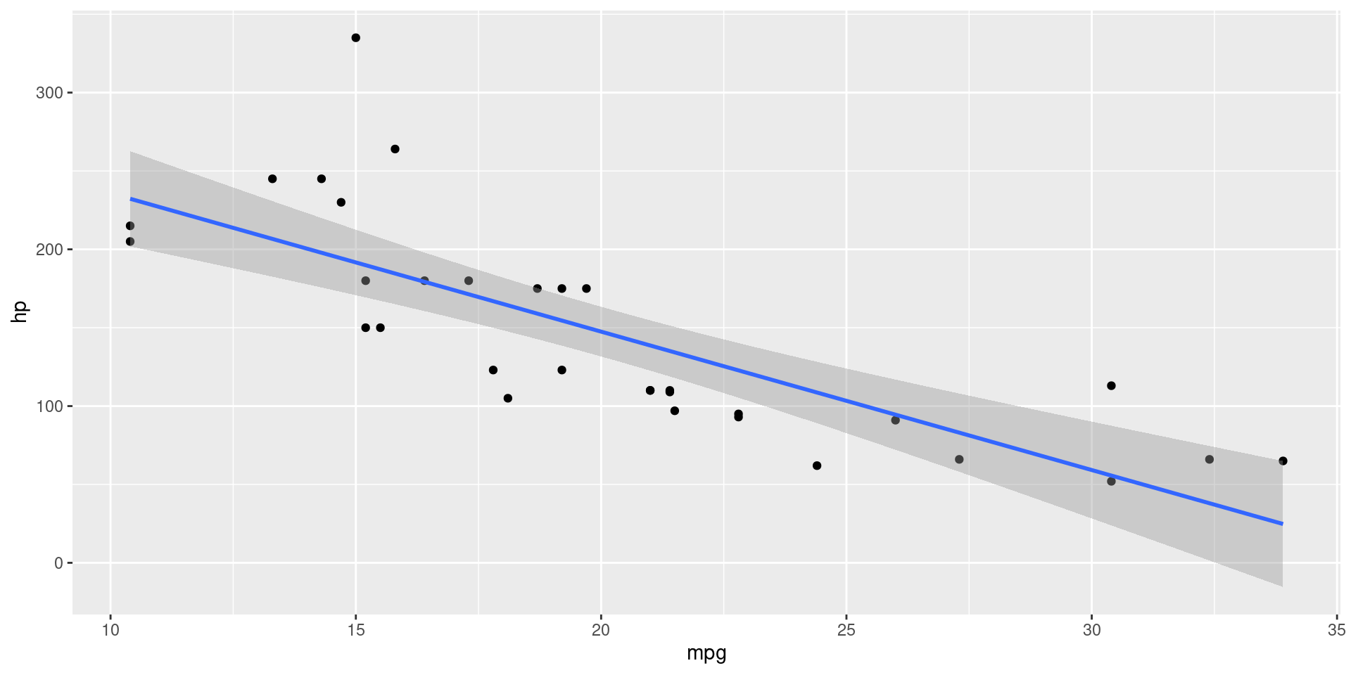
Regression Line
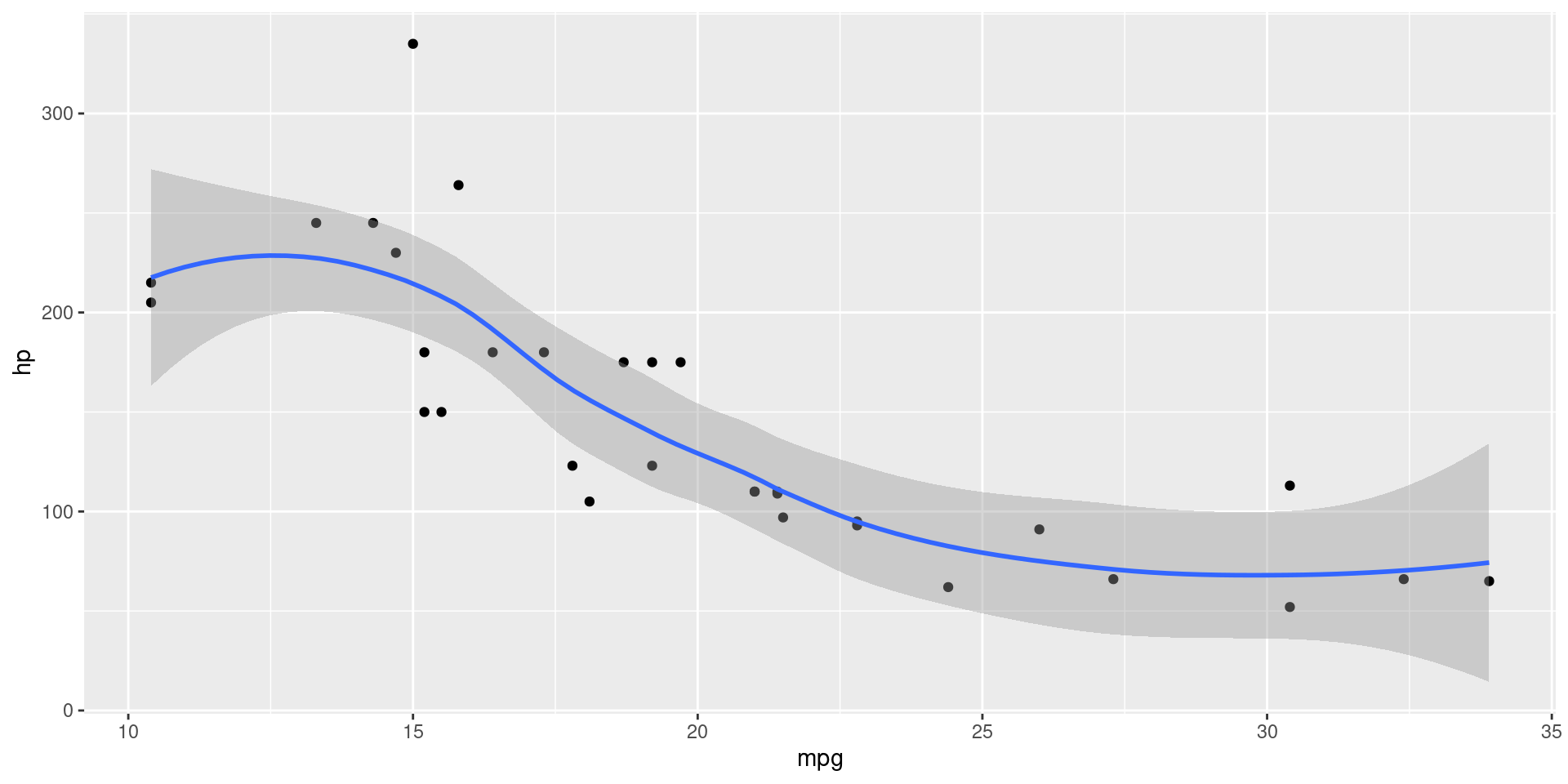
LOESS Line
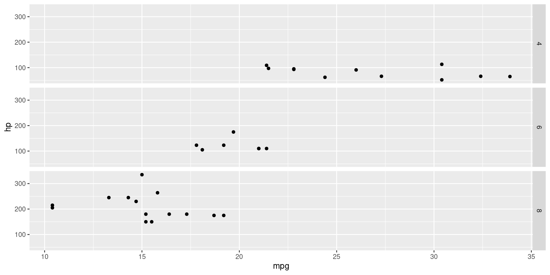
Facet
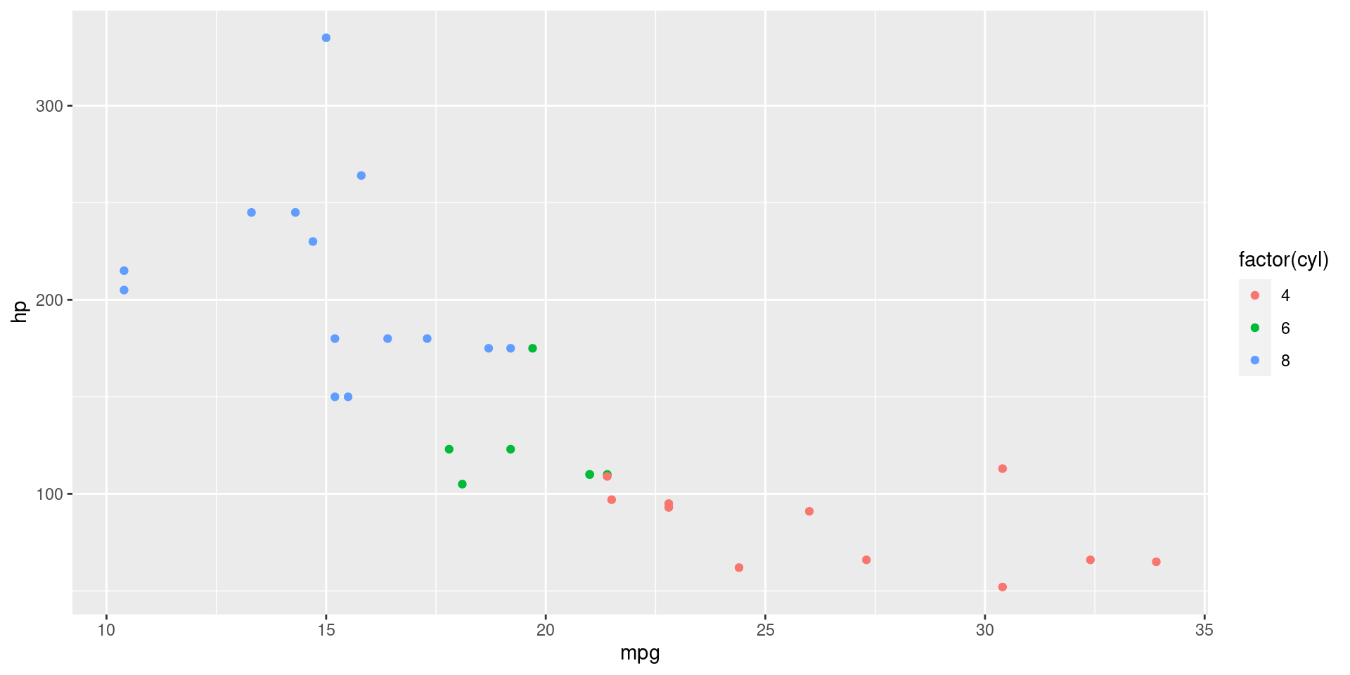
Mapping
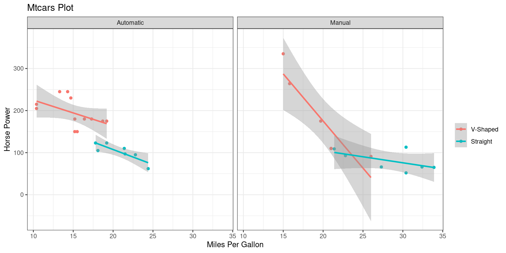
Advanced Example
Advanced Example
Base Plot
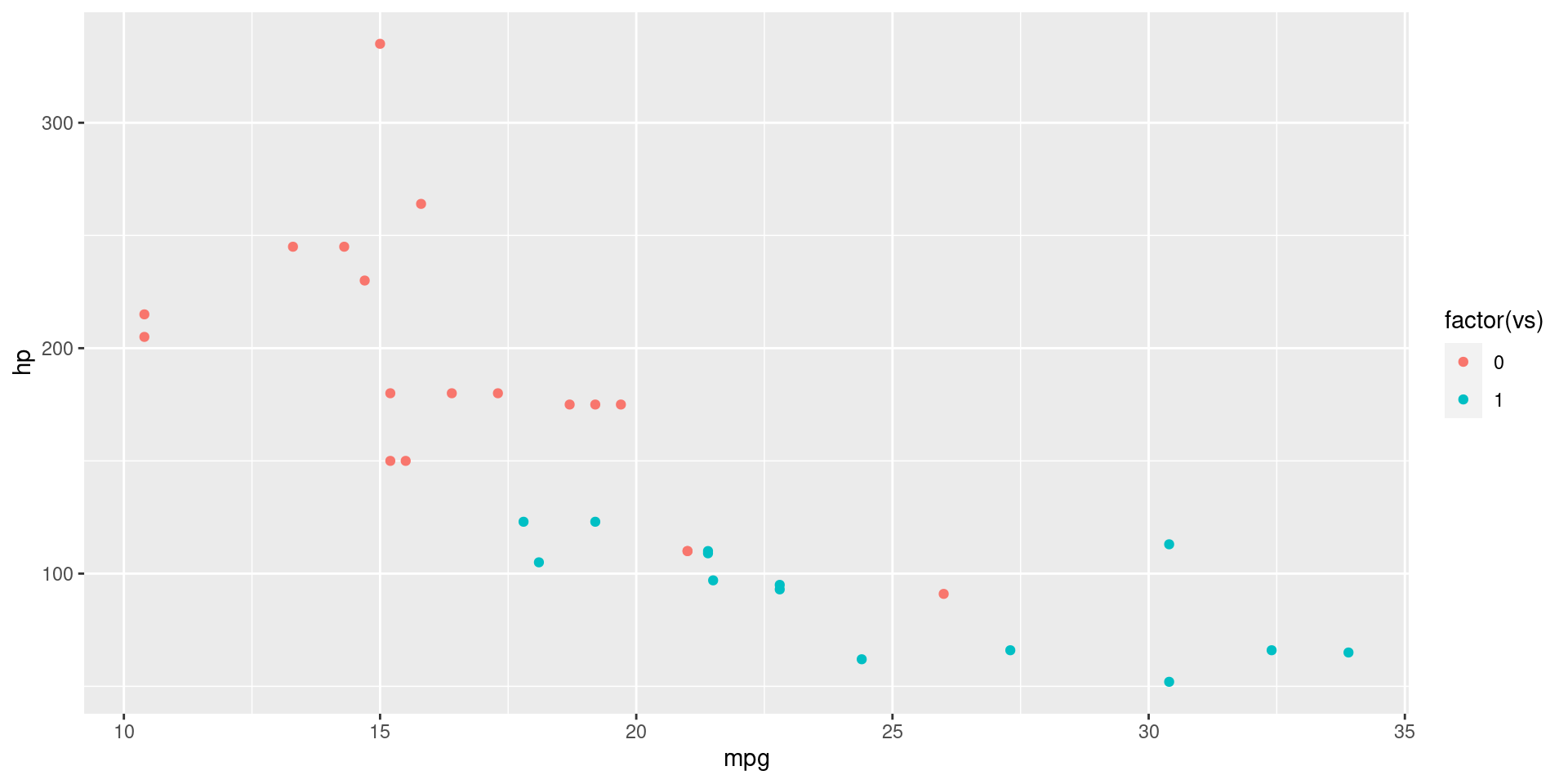
Scatter Plot
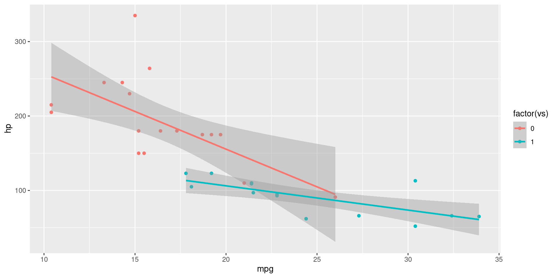
Add Regression Line
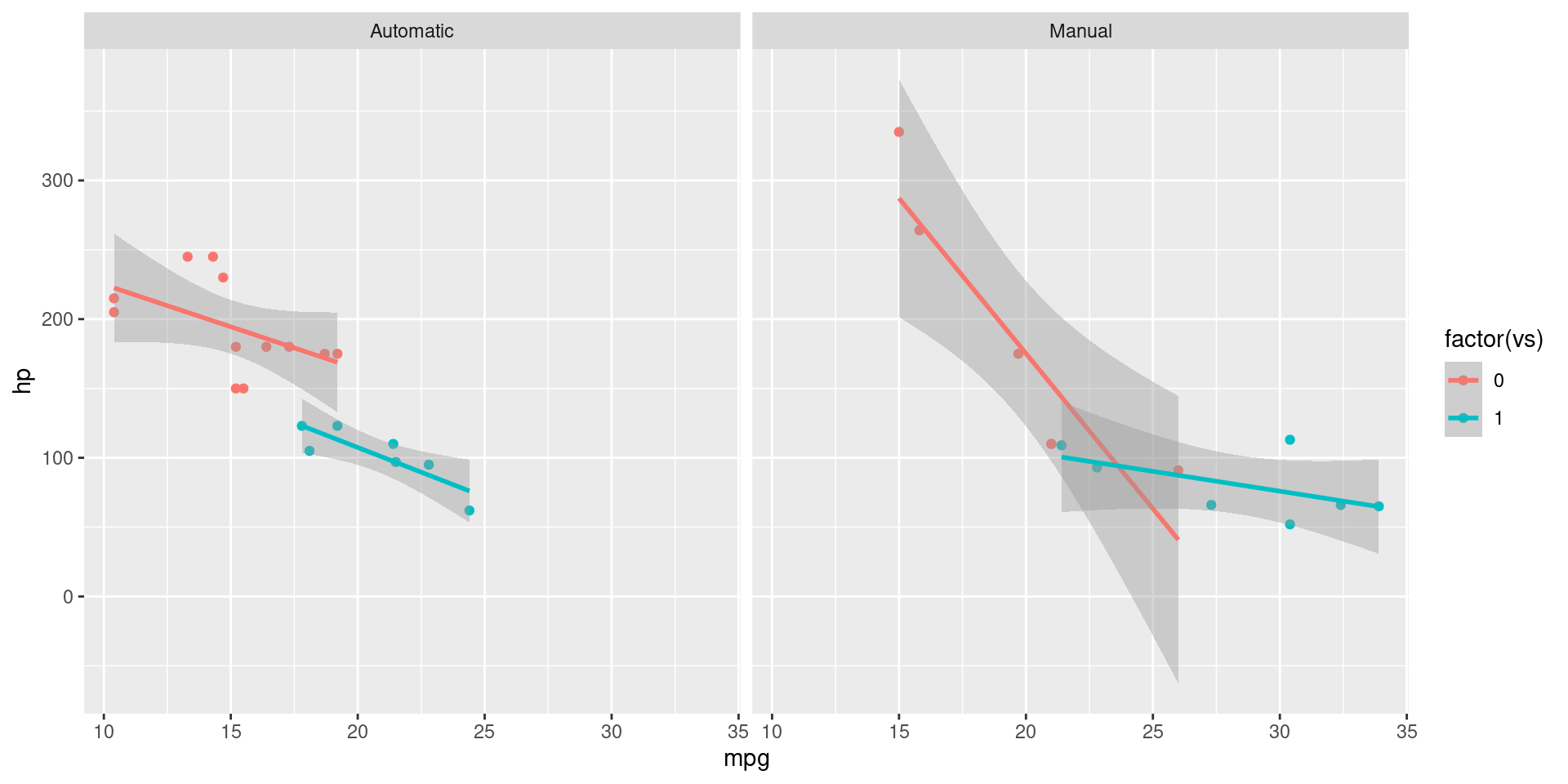
Split The Plot
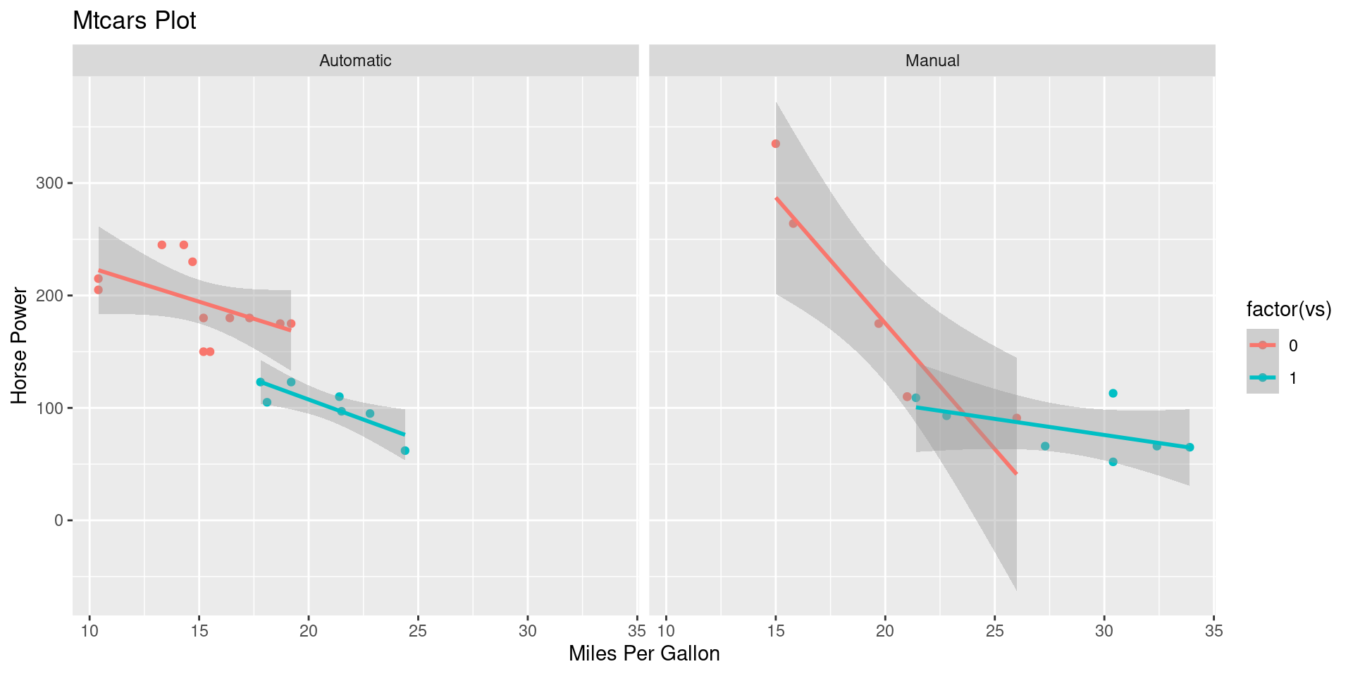
Change the Labels
Adjust the Legend
Change the theme
Plot Code

Plot Code
Plot Code
Plot Code
Plot Code
Plot Code
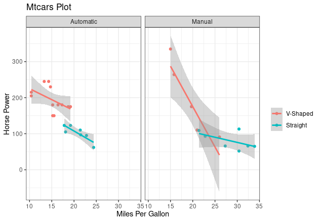
ggplot(mtcars,
       aes(mpg, hp,
color = factor(vs))) +
geom_point()+
geom_smooth(method = "lm") +
facet_grid(cols = vars(am),
labeller = as_labeller(c(
`1` = "Manual",
`0` = "Automatic"))) +
ggtitle("Mtcars Plot") +
xlab("Miles Per Gallon") +
ylab("Horse Power") +
scale_color_discrete(
labels = c("V-Shaped", "Straight"),
name = "")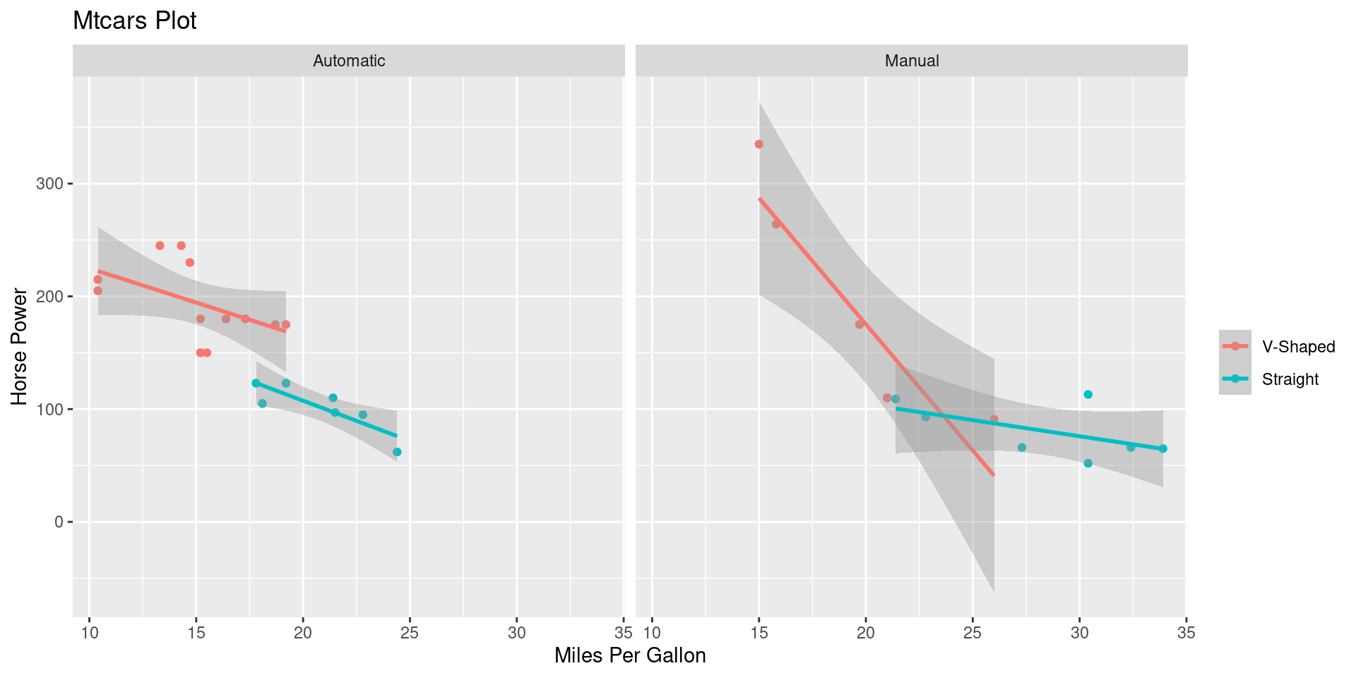
Plot Code
ggplot(mtcars,
       aes(mpg, hp,
           color = factor(vs))) +
geom_point()+
geom_smooth(method = "lm") +
facet_grid(cols = vars(am),
labeller = as_labeller(c(
`1` = "Manual",
`0` = "Automatic"))) +
ggtitle("Mtcars Plot") +
xlab("Miles Per Gallon") +
ylab("Horse Power") +
scale_color_discrete(
labels = c("V-Shaped", "Straight"),
name = "") +
theme_bw()