```{r setup, include=FALSE}
library(tidyverse)
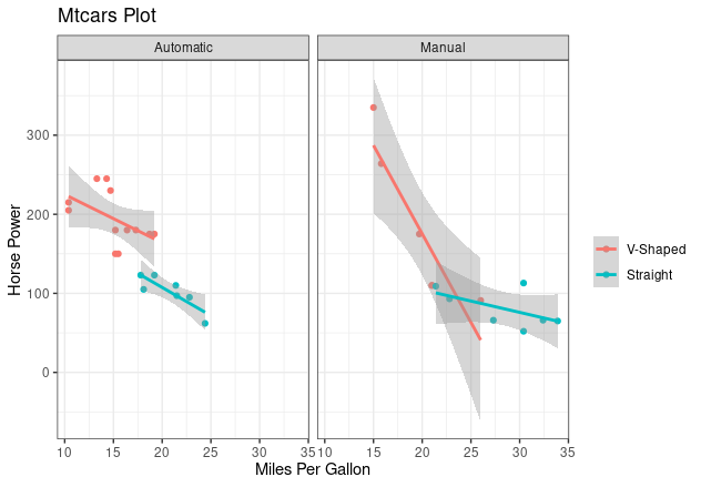
adv_plot <- ggplot(mtcars, aes(mpg, hp, color = factor(vs))) +
geom_point() +
geom_smooth(method = "lm") +
facet_grid(cols = vars(am),
labeller = as_labeller(c(`1` = "Manual",
`0` = "Automatic"))) +
ggtitle("Mtcars Plot") +
xlab("Miles Per Gallon") + ylab("Horse Power") +
scale_color_discrete(labels = c("V-Shaped", "Straight"),
name = "") +
theme_bw()
```
## Presentation Online
Presentation:
[www.inqs.info/files/hiss_3/hiss_3.html](https://www.inqs.info/files/hiss_3/hiss_3.html)
RMD:
[www.inqs.info/files/hiss_3/hiss_3.qmd](https://www.inqs.info/files/hiss_3/hiss_3.qmd)
Website:
[www.inqs.info](https://www.inqs.info)
Email:
iquin002\@ucr.edu
# Data Cleaning
## dplyr
- Known as the Grammar of Data Manipulation
- [dplyr.tidyverse.org](https://dplyr.tidyverse.org/)
## dplyr Functions
- `mutate()` adds new variables
- `select()` selects variables
- `filter()` filters data
- `if_else()` conditional function that returns 2 values
- `group_by()` a dataset is grouped by factors
- `summarise()` provides summaries of data
## tidyr
- Used to create tidy data
- [tidyr.tidyverse.org](https://tidyr.tidyverse.org/)
## tidyr Functions
- `pivot_longer()` (formerly `gather()`) transforms the data from wide to long
- `pivot_wider()` (formerly `spread()`) transforms the data from long to wide
- `separate()` separates a one variable to multiple variables
- `unite()` merge multiple variable to one variable
## Pipe Operator `%>%`
- The pipe operator is the real power of tidyverse.
- It takes the output of a function and uses it as input for another function.
- Tidyverse works best when data frames (tibbles) are used a inputs.
## Data Set
- We will work on manipulating the `mtcars` data set
- Below prints out the code:
::: fragment
```{r}
mtcars %>%
head(n=3)
```
:::
## `mutate()`
- Adds a new variable to a data frame
- Example:
::: fragment
```{r}
#| code-line-numbers: "|2"
mtcars %>%
mutate(log_mpg=log(mpg)) %>%
head(n=3)
```
:::
## `mutate()`
- Each argument adds a new variable added
- Example:
::: fragment
```{r}
#| code-line-numbers: "|2"
mtcars %>%
mutate(log_mpg=log(mpg),log_hp=log(hp)) %>%
head(n=3)
```
:::
## `select()`
-This selects the variables to keep in the data frame
-Example:
::: fragment
```{r}
#| code-line-numbers: "|3"
mtcars %>%
mutate(log_mpg=log(mpg),log_hp=log(hp)) %>%
select(mpg,log_mpg,hp,log_hp) %>%
head(n=3)
```
:::
## `filter()`
- Selects observations that satisfy a condition
- Example:
::: fragment
```{r}
#| code-line-numbers: "|4"
mtcars %>%
mutate(log_mpg=log(mpg),log_hp=log(hp)) %>%
select(mpg,log_mpg,hp,log_hp) %>%
filter(log_hp<5) %>%
head(n=3)
```
:::
## `if_else()`
- A function that provides T (1) if the condition is met and F (0) otherwise
- Example:
::: fragment
```{r}
#| code-line-numbers: "|5"
mtcars %>%
mutate(log_mpg=log(mpg),log_hp=log(hp)) %>%
select(mpg,log_mpg,hp,log_hp) %>%
filter(log_hp<5) %>%
mutate(hilhp=if_else(log_hp>mean(log_hp),1,0)) %>%
head(n=3)
```
:::
## `group_by()`
- This groups the data frame
- Example:
::: fragment
```{r}
#| code-line-numbers: "|6"
mtcars %>%
mutate(log_mpg=log(mpg),log_hp=log(hp)) %>%
select(mpg,log_mpg,hp,log_hp) %>%
filter(log_hp<5) %>%
mutate(hilhp=if_else(log_hp>mean(log_hp),1,0)) %>%
group_by(hilhp) %>%
head(n=3)
```
:::
## `summarise()`
- Creates summary statistics for variables
::: fragment
```{r}
#| code-line-numbers: "|7-8"
mtcars %>%
mutate(log_mpg=log(mpg),log_hp=log(hp)) %>%
select(mpg,log_mpg,hp,log_hp) %>%
filter(log_hp<5) %>%
mutate(hilhp=if_else(log_hp>mean(log_hp),1,0)) %>%
group_by(hilhp) %>%
summarise(mean_mpg=mean(mpg),mean_lmpg=mean(log_mpg),
sd_mpg=sd(mpg),sd_lmpg=sd(log_mpg)) %>%
head(n=3)
```
:::
# Wide to Long Example
## Wide to Long Data Example
We work on converting data from wide to long using the functions in the tidyr package. For many statistical analysis, long data is necessary.
## Load Data
Use the `read_csv()` to read `data_3_4.csv` into an object called `data1`;
```{r,message=F}
data1 <- read_csv(file="http://www.inqs.info/files/hiss_3/data_3_4.csv")
```
## Wide Data
```{r}
#| echo: false
names(data1)
head(data1)
```
## Long Data
```{r,include=FALSE}
data1_long <- data1 %>% pivot_longer(`v1/mean`:`v4/median`,"measurement","value") %>%
separate(measurement,c("time","stat"),sep="/") %>%
pivot_wider(names_from = stat,values_from = value)
```
```{r}
#| echo: false
head(data1_long, n = 10)
```
## `pivot_longer()`
- The `pivot_longer()` function grabs the variables that repeated in an observation places them in one variable:
::: fragment
```{r}
#| code-line-numbers: "|2"
data1 %>%
pivot_longer(cols=`v1/mean`:`v4/median`,names_to = "measurement",values_to = "value") %>%
head()
```
:::
## `separate()`
- The `separate()` function will separate a variable to multiple variables:
::: fragment
```{r}
#| code-line-numbers: "|3"
data1 %>%
pivot_longer(cols=`v1/mean`:`v4/median`,names_to = "measurement",values_to = "value") %>%
separate(col=measurement,into=c("time","stat"),sep="/") %>%
head()
```
:::
## `pivot_wider()`
- The `pivot_wider()` function then converts long data to wide data.
::: fragment
```{r}
#| code-line-numbers: "|4"
data1 %>%
pivot_longer(`v1/mean`:`v4/median`,"measurement","value") %>%
separate(measurement,c("time","stat"),sep="/") %>%
pivot_wider(names_from = stat,values_from = value) %>%
head()
```
:::
# Graphics
## ggplot2
- Known as the Grammar of Graphics
- [ggplot2.tidyverse.org](https://ggplot2.tidyverse.org/)
## Basics
- ggplot2 creates a plot by layering graphical elements on top of a plot
- A base plot is created with the data
- The data must be a data frame or tibble
- Additional layers are added to base plot with `+` sign
## Using ggplot2
- Create Base Plot
- Add geometrical Elements
- Customize Plot
- Google
## Base Plot
- A base plot is created using `ggplot2()`
- `data`: specifies data frame to construct the base plot
- `mapping`: specifies the aesthetic mapping for the plot
- `aes()`: creates the mapping function
::: fragment
```{r}
base_plot <- ggplot(mtcars, aes(x=mpg))
```
:::
## Base Plot
```{r}
base_plot
```
## Univariate
- Histograms
- `geom_histogram()`
- Density Plots
- `geom_density()`
- qq plot
- `geom_qq()`
- `geom_qq_line()`
## Histograms
```{r}
base_plot + geom_histogram()
```
## Density Plot
```{r}
base_plot + geom_density()
```
## QQ Plot
```{r}
ggplot(mtcars, aes(sample = mpg)) +
geom_qq() +
geom_qq_line()
```
## Bivariate
- Scatter Plot
- `geom_point()`
- Line Plot
- `geom_line()`
## Bivariate Base Plot
```{r}
base_plot2 <- ggplot(mtcars, aes(x=mpg, y = hp))
base_plot2
```
## Scatter Plot
```{r}
base_plot2 + geom_point()
```
## Line Plot
```{r}
base_plot2 + geom_line()
```
## Line & Scatter Plot
```{r}
base_plot2 +
geom_point() +
geom_line()
```
## Special Cases
::: columns
::: {.column width="50%"}
### Bivariate
- Heat Map
- `geom_bin2d()`
- Contour Map
- `geom_density_2d()`
:::
::: {.column width="50%"}
### Trivariate
- Heat Map
- `geom_contour_filled()`
- Contour Map
- `geom_contour()`
:::
:::
## Heat Map
```{r}
base_plot2 + geom_bin2d()
```
## Contour Map
```{r}
base_plot2 +
geom_density2d()
```
## Trend Lines
- Regression Line
- `geom_smooth(method = "lm")`
- LOESS
- `geom_smooth()`
## Regression Line
```{r}
base_plot2 +
geom_point() +
geom_smooth(method = "lm")
```
## LOESS Line
```{r}
base_plot2 +
geom_point() +
geom_smooth()
```
## Grouping Plots
- Faceting: Facet allows you to subset the data by a categorical variable
- `facet_grid()`
- `facet_wrap()`
- Grouping can be done within the mapping function: `aes()`
- `color`
- `group`
- `shape`
## Facet
```{r}
ggplot(mtcars, aes(x = mpg, y = hp)) +
geom_point() +
facet_grid(vars(cyl))
```
## Mapping
```{r}
ggplot(mtcars, aes(x = mpg, y = hp, col = factor(cyl))) +
geom_point()
```
## Customization
- Title
- `ggtitle()`
- Labels
- X Label: `xlab()`
- Y Label: `ylab()`
## Themes
- The `theme()` function allows you to change any component in the plot
- ggplot2 has several prebuilt themes:
- `theme_bw()`
- `theme_void()`
- Legends can be adjusted using the `scale_XX_YY()`
- `XX`: the type grouping factor
- `YY`: the type variable
## Advanced Example {auto-animate="true"}
{fig-align="center"}
## Advanced Example {auto-animate="true"}
::: columns
::: {.column width="50%"}

:::
::: {.column width="50%"}
- Base Plot
- Scatter Plot
- Add Regression Line
- Split The Plot
- Change the Labels
- Adjust the Legend
- Change the theme
:::
:::
## Plot Code {auto-animate="true" visibility="uncounted"}
::: columns
::: {.column width="60%"}
```{r}
#| eval: false
ggplot(mtcars,
aes(mpg, hp,
color = factor(vs)))
```
:::
::: {.column width="40%"}
```{r}
#| echo: false
ggplot(mtcars, aes(mpg, hp, color = factor(vs)))
```
:::
:::
## Plot Code {auto-animate="true" visibility="uncounted"}
::: columns
::: {.column width="60%"}
```{r}
#| eval: false
ggplot(mtcars,
aes(mpg, hp,
color = factor(vs))) +
geom_point()
```
:::
::: {.column width="40%"}
```{r}
#| echo: false
ggplot(mtcars, aes(mpg, hp, color = factor(vs))) +
geom_point()
```
:::
:::
## Plot Code {auto-animate="true" visibility="uncounted"}
::: columns
::: {.column width="60%"}
```{r}
#| eval: false
ggplot(mtcars,
aes(mpg, hp,
color = factor(vs))) +
geom_point()+
geom_smooth(method = "lm")
```
:::
::: {.column width="40%"}
```{r}
#| echo: false
ggplot(mtcars, aes(mpg, hp, color = factor(vs))) +
geom_point()+
geom_smooth(method = "lm")
```
:::
:::
## Plot Code {auto-animate="true" visibility="uncounted"}
::: columns
::: {.column width="60%"}
```{r}
#| eval: false
ggplot(mtcars,
aes(mpg, hp,
color = factor(vs))) +
geom_point()+
geom_smooth(method = "lm") +
facet_grid(cols = vars(am),
labeller = as_labeller(c(
`1` = "Manual",
`0` = "Automatic")))
```
:::
::: {.column width="40%"}
```{r}
#| echo: false
ggplot(mtcars, aes(mpg, hp, color = factor(vs))) +
geom_point()+
geom_smooth(method = "lm") +
facet_grid(cols = vars(am),
labeller = as_labeller(c(`1` = "Manual",
`0` = "Automatic")))
```
:::
:::
## Plot Code {auto-animate="true" visibility="uncounted"}
::: columns
::: {.column width="60%"}
```{r}
#| eval: false
ggplot(mtcars,
aes(mpg, hp,
color = factor(vs))) +
geom_point()+
geom_smooth(method = "lm") +
facet_grid(cols = vars(am),
labeller = as_labeller(c(
`1` = "Manual",
`0` = "Automatic"))) +
ggtitle("Mtcars Plot") +
xlab("Miles Per Gallon") +
ylab("Horse Power")
```
:::
::: {.column width="40%"}
```{r}
#| echo: false
ggplot(mtcars, aes(mpg, hp, color = factor(vs))) +
geom_point()+
geom_smooth(method = "lm") +
facet_grid(cols = vars(am),
labeller = as_labeller(c(`1` = "Manual",
`0` = "Automatic"))) +
ggtitle("Mtcars Plot") +
xlab("Miles Per Gallon") +
ylab("Horse Power")
```
:::
:::
## Plot Code {auto-animate="true" visibility="uncounted"}
::: columns
::: {.column width="60%"}
```{r}
#| eval: false
ggplot(mtcars,
aes(mpg, hp,
color = factor(vs))) +
geom_point()+
geom_smooth(method = "lm") +
facet_grid(cols = vars(am),
labeller = as_labeller(c(
`1` = "Manual",
`0` = "Automatic"))) +
ggtitle("Mtcars Plot") +
xlab("Miles Per Gallon") +
ylab("Horse Power") +
scale_color_discrete(
labels = c("V-Shaped", "Straight"),
name = "")
```
:::
::: {.column width="40%"}
```{r}
#| echo: false
ggplot(mtcars, aes(mpg, hp, color = factor(vs))) +
geom_point()+
geom_smooth(method = "lm") +
facet_grid(cols = vars(am),
labeller = as_labeller(c(
`1` = "Manual",
`0` = "Automatic"))) +
ggtitle("Mtcars Plot") +
xlab("Miles Per Gallon") +
ylab("Horse Power")+
scale_color_discrete(
labels = c("V-Shaped", "Straight"),
name = "")
```
:::
:::
## Plot Code {auto-animate="true" visibility="uncounted"}
::: columns
::: {.column width="60%"}
```{r}
#| eval: false
ggplot(mtcars,
aes(mpg, hp,
color = factor(vs))) +
geom_point()+
geom_smooth(method = "lm") +
facet_grid(cols = vars(am),
labeller = as_labeller(c(
`1` = "Manual",
`0` = "Automatic"))) +
ggtitle("Mtcars Plot") +
xlab("Miles Per Gallon") +
ylab("Horse Power") +
scale_color_discrete(
labels = c("V-Shaped", "Straight"),
name = "") +
theme_bw()
```
:::
::: {.column width="40%"}
```{r}
#| echo: false
ggplot(mtcars, aes(mpg, hp, color = factor(vs))) +
geom_point()+
geom_smooth(method = "lm") +
facet_grid(cols = vars(am),
labeller = as_labeller(c(
`1` = "Manual",
`0` = "Automatic"))) +
ggtitle("Mtcars Plot") +
xlab("Miles Per Gallon") +
ylab("Horse Power")+
scale_color_discrete(
labels = c("V-Shaped", "Straight"),
name = "") +
theme_bw()
```
:::
:::
## Final Thoughts
- Google is your friend!
- Practice!
- Read the documentation!
- Utilize Cheatsheets!
## Resources
-
-
-
-