Data Cleaning in R

Published

September 28, 2024

Modified

October 23, 2024

Data manipulation consists of transforming a data set to be analyzed. Certain statistical methods require data sets to be formatted in a certain way before you can apply a certain function¹. Other times, you will need to transform the data set to present to stakeholder. Therefore, being able to transform a data set is essential.

Warnings Suppressed

In order to keep the page concise, the warning messages have been suppressed. These warnings were produced because functions were applied to incorrect inputs, ie \(\sqrt{A}\). Therefore, you may see NA as the output. There is nothing wrong with the code, it is just that the input was not valid, but R still completed the task.

Tidyverse

Tidyverse is a set of packages that make data manipulation much easier. These are functions that many individuals from the R community find useful to use for data analysis. Many of the functions are descriptively named for easy remembrance. If you haven’t done so, install tidyverse:

install.packages("tidyverse")

Then load tidyverse into R:

library(tidyverse)

This will load the main Tidyverse packages: ggplot2, tibble, tidyr, readr, purr, dplyr, stringr, and forcats.

Loading Data

There are three methods to load a data set in R: using base R, using Tidyverse, or using RStudio. While it is important to understand how the code works to load a data set, I recommend using RStudio to import the data. It does all the work for you. Additionally, if you decide to use Tidyverse packages, RStudio will provide corresponding code for a particular file.

To import a data set using RStudio, head over to the environment tab (usually in the upper right hand pane) and click on the Import Dataset button. A pop-up window should look something like below.

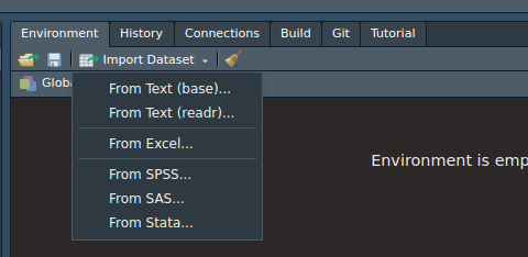
Notice how there are several options to load a data set. Depending on the format, you may want to choose one of those options. Next, notice how there are 2 “From Text”. This is because it will load text data using either Base R packages or the readr package from tidyverse. Either works, but the readr package provides the necessary code to load the data set in the window. The other one provides the code in the console.

CSV Files

A CSV file is a type of text file that where the values are separated from commas. It is very common file that you will work with. Here I will provide the code necessary to import a CSV file using either Base R or readr package code.

Base R

read.csv("FILE_NAME_AND_LOCATION")

`readr` package

read_csv("FILE_NAME_AND_LOCATION")

Notice that the functions are virtually the same.

For This Page

You will need to download and extract this zip file to conduct the analysis in the chapter. The code below will load the data sets you need:

data1 <- read_csv("data/data_3_1.csv")
data2 <- read_csv("data/data_3_2.csv")
data3 <- read_csv("data/data_3_3.csv")
data4 <- read_csv("data/data_3_6.csv")
data5 <- read_csv("data/data_3_7.csv")
data6 <- read_csv("data/data_3_5.csv")
data7 <- read_csv("data/data_3_4.csv")

Make sure to change the file location as needed.

The Pipe Operator `|>`

The main benefit of the pipe operator is to make the code easier to read. The base pipe |> was added in R 4.0. What the pipe operator, |>, does is that it will take the output from a previous function and it will use it as the input for the next function. This prevents us from nesting functions together and overwhelm us with numerous parentheses and commas. To practice, pipe data into the glimpse().

data1 |> glimpse()

#> Rows: 1,000
#> Columns: 10
#> $ ID1  <chr> "A2b6115fd", "Ac51c9cf1", "A7534d3a0", "A73fc5642", "Ae020e4bd", …
#> $ cat1 <chr> "A", "A", "A", "A", "C", "A", "A", "C", "B", "C", "B", "B", "A", …
#> $ cat2 <chr> "E", "D", "F", "F", "E", "D", "E", "F", "E", "E", "F", "E", "E", …
#> $ var1 <dbl> 1.1541672, -0.3667030, -0.4203357, -2.0006336, 0.6970417, 0.46690…
#> $ var2 <dbl> 4, 3, 6, 5, 3, 4, 5, 0, 5, 3, 3, 8, 4, 5, 2, 5, 7, 7, 5, 1, 4, 3,…
#> $ var3 <dbl> 2.87981553, 0.06397162, -1.04021753, -0.31355281, 0.52613439, 2.4…
#> $ var4 <dbl> 3.53845785, 1.07279559, 0.22632480, 0.02128418, 2.97936180, 1.853…
#> $ var5 <dbl> -3.1827969, -3.1827969, -3.1827969, -3.1827969, 6.0601967, -3.182…
#> $ var6 <dbl> 0, 0, 0, 0, 0, 0, 0, 0, 0, 0, 0, 0, 0, 0, 0, 0, 0, 0, 0, 0, 0, 0,…
#> $ var7 <dbl> 1, 0, 0, 0, 0, 0, 1, 1, 0, 1, 0, 1, 0, 1, 1, 0, 1, 0, 1, 0, 1, 1,…

The glimpse() provides basic variable information about data1. I recommend practice reading the code in plain English to help you understand how these functions.

Data Transformation

This section focuses on manipulating the data to obtain basic statistics, such as obtaining the mean for different categories. Many of the functions used here are from the dplyr package.

Summarizing Data

Summarizing Data is one of the most important thing in statistics. First, let’s get the mean for all the variables in data1. This is done by using the summarize_all(). All you need to do is provide the function you want R to provide. Pipe data1 into the summarize_all() and specify mean in the function.

data1 |> summarise_all(mean)

Notice how some values are NA, this is because the variables are character data types. Therefore, it will not be able to compute the mean. Now find the standard deviation for the data set.

data1 |> summarise_all(sd)

Now lets create a frequency table for the cat1 variable in data1. use the count() and specify the variable you are interested in:

data1 |> count(cat1)

Now, repeat for cat2 in data1:

data1 |> count(cat2)

Grouping

Summarizing data is great, but sometimes you may want to group data and obtain summary statistics for those groups. This is done by using the group_by() and specify which variable you want to group. Try grouping data1 by cat1:

data1 |> group_by(cat1)

Great! You now have grouped data; however, this is not helpful (note everything looks the same). We can use this output and summarize the groups. All we need to do is pipe the output to the summarise_all(). Group data1 by cat1 and find the mean:

data1 |> group_by(cat1) |> summarise_all(mean)

If we want to group by two variables, all we need to do is specify both variables in the group_by(). Group data1 by cat1 and cat2 then find the mean:

data1 |> group_by(cat1,cat2) |> summarise_all(mean)

Now, instead of finding the mean for all variables in a data set, we are only interested in viewing var1. We can use the summarise() and type the R code for finding the mean for the particular variable. Group data1 by cat1 and find the mean for var1:

data1 |> group_by(cat1) |> summarise(mean(var1))

Subsets

On occasion, you may need to create a subset of your data. You may only want to work with one part of your data. To create a subset of your data, use the filter() to create the subset. This will select the rows that satisfy a certain condition. Create a subset of data1 where only the positive values of var1 are present. Use the filter() and state var1>0.

data1 |> filter(var1>0)

If you know which rows you want, you can use the slice() and specify the rows as a vector. Create a subset of data1 and select the rows 100 to 200 and 300 to 400.

data1 |> slice(c(100:200, 300:400))

If you need random sample of your data1, use the slice_sample(n = N) and specify the number you want. It will create a data set of randomly selected rows. Create a random sample of data1 of 100 rows.

data1 |>  slice_sample(n = 100)

If you want a random sample that is proportion of your original data size, use the slice_sample(prop = X). Specify the proportion that you want from the data. Create a random sample of data1 that is only 2/7th of the original size.

data1 |> slice_sample(prop = 2/7)

Creating Variables

Some times you may need to transform variables to a new variable. This can be done by using the mutate() where you specify the name of the new variable and set equal to the transformation of other variables. Using the data2 data set, create a new variable called logvar1 and set that to the log of va1.

data2 |> mutate(logvar1 = log(va1))

The mutate() allows you to create multiple new variables at once. Id addition to logvar1, create a new variable called sqrtvar2 and set that equal to the square root of va2.

data2 |> mutate(logvar1 = log(va1), 
                sqrtvar2 = sqrt(va2))

If you want to create categorical variables, use the mutate() and the if_else(). The if_else() requires three arguments: condition argument, true argument, and false argument. The first argument requires a condition that will return a logical value. If true, then R will assign what is stated in the true argument, otherwise R will assign what is in the false argument. To begin, find the median of va1 from data2 and assign it to medval.

medval <- data2$va1 |> median()

No create a new variable called diva1 where if va1 is greater than the median of va1, assign it “A”, otherwise assign it “B”.

data2 |> mutate(diva1=if_else(va1>medval,"A","B"))

Merging Datasets

One of the last thing is to go over how to merge data sets together. To merge the data sets, we use the full_join(). The full_join() needs two data sets (separated by commas) and the by argument which provides the variables needed (must be the same name for each data set) to merge the data sets. Merge data1 and data2 with the variable ID1.

full_join(data1, data2, by = "ID1")

The full_join() allows you to merge data sets using two variables instead of one. All you need to do is specify by argument with a vector specifying the arguments. Merge data2 and data3 by ID_1 and ID_2.

full_join(data2, data3, by = c("ID_1","ID_2"))

Reshaping Data

This section focuses on reshaping the data to prepare it for analysis. For example, to conduct longitudinal data analysis, you will need to have long data. Reshaping data may be with converting data from wide to long, converting back from long to wide, splitting variables, splitting rows and merging variable. The functions used in this lesson are from the tidy package

Wide to Long Data

Converting data from wide to long is necessary when the data looks like data4, view data4:

data4

Let’s say data4 represents biomarker data. Variable ID1 represents a unique identifier for the participant. Then X1, X2, X3, and X4 represents a value collected for a participant at different time point. This is know as repeated measurements. This data is considered wide because the repeated measurements are on the same row. To make it long, the repeated measurements must be on the same column.

To convert data from long to wide, we will use the pivot_longer() with the first argument taking variables of the repeated measurements, c(X1:X4) or X1:X4, second you will need to specify the names_to argument which specifies the variable name to store the long variables, lastly you will need to specify the values_to argument that specifies variable to store the values in the long data set. Convert the data4 to long and name the variable names column "measurement", and values column "value".

data4 |> pivot_longer(X1:X4, 
                      names_to = "measurement", 
                      values_to = "value")

Long to Wide

If you need to convert data from long to wide, use the pivot_wider(). You will need to specify the names_from argument which specifies the variable names for the wide data set, and you will need to specify the values_from argument that specifies variable that contains the values in the long data set. Convert data5 from long to wide data. Note, you must specify the arguments for this function.

data5 |> pivot_wider(names_from = measurement, 
                     values_from = value)

Spliting Variables

Before we begin, look at data6:

data6

Notice how the merge variable has two values separated by “/”. If we need to split the variable into two variables, we need to specify the separate(). All you need to specify is the variable you need to split, the name of the 2 new variables, in a character vector, and how to split the variable "/". Split the variable merge in data6 to two new variables called X1 and X2.

data6 |> separate(merge, c("X1", "X2"), "/")

Splitting Rows

The variable merge in data6 was split into different variables before, now instead of variables, let’s split it into different rows instead. To do this, use the separate_rows(). All you need to specify the variable name and the sep argument (must state the argument). Split the merge variable from data6 into different rows.

data6 |> separate_rows(merge, sep = "/")

Merging Rows

If you need to merge variables together, similar to the merge variable, use the unite(). All you need to do is specify the variables to merge, the col argument which specifies the name of the new variable (as a character), and the sep argument which indicates the symbol for separate value, as a character. Note, you need to specify the bot the col argument and sep argument. Merge variable X3 and X4 in data6 to a new variable called merge2 and have the separator be a hyphen.

data6 |> unite(X3, X4, col = "merge2", sep="-")

Applied Example

Here is an applied example where you will use what you learned from the previous lesson and convert data7 into data8. data7 has a wide data format which contains time points labeled as vX, where X represents the time point number. At each time point, the mean, sd, and median was taken. You will need to convert the data to long where each row represents a new time point, and each row will have 3 variables representing the mean, sd, and median. View both data7 and data8 to have a better idea on what is going on. Remember you need to convert data7 to data8.

data7

data8

Now that you viewed the data set, type the code to convert data7 to data8. Try working it out before you look at the solution.

data7 |> pivot_longer(`v1/mean`:`v4/median`,
                      names_to = "measurement",
                      values_to = "value") |> 
          separate(measurement, c("time","stat"), sep="/") |> 
          pivot_wider(names_from = stat, values_from = value)

Footnotes

Linear Mixed-Effects Models.↩︎