# This code will load the R packages we will use
install.packages(c("csucistats"),
                 repos = c("https://inqs909.r-universe.dev", "https://cloud.r-project.org"))
library(csucistats)
library(tidyverse)

# Uncomment and run for categorical plots
csucistats::install_plots()
library(ggtricks)
library(ggmosaic)
library(waffle)

# Uncomment and run for themes
# csucistats::install_themes()
# library(ThemePark)
# library(ggthemes)Categorical Data
Descriptive summaries & visualizations (freq, proportion, crosstabs, bar/pie/mosaic/waffle)
A student‑friendly reference with concise explanations, runnable examples, and copy‑paste templates for analyzing and visualizing categorical data in R.
1 Learning goals
- Recognize and work with categorical variables in R.
- Summarize categories using frequencies and proportions (a.k.a. relative frequency).
- Create standard plots for categorical data: bar, stacked bar, pie, mosaic, and waffle.K
- Read and interpret cross‑tabulations (two‑way tables) with row/column/table proportions.
Tip
Use the Copy button on each code chunk. Many chunks include a template version followed by a worked example.
2 Google Colab Setup
Important
Google Colab recently updated its R version, therefore, the categorical plots may not install. Comment (Add a # in front of the line) the code to csucistats::install_plots(), library(ggtricks), library(ggmosaic), and library(waffle) if it is not working.
2.1 Data for this handout
We will use the Great American Coffee Taste Test survey data from TidyTuesday. Below is a subset of the data.
Code
coffee <- read_csv("https://raw.githubusercontent.com/rfordatascience/tidytuesday/master/data/2024/2024-05-14/coffee_survey.csv")2.2 Using the templates: what to change
Use this legend whenever you see a Template code block.
DATA→ replace with your data frame/tibble name (e.g.,coffee).VAR→ replace with the single categorical variable you want (e.g.,caffeine).- In
ggplot(DATA, aes(x = VAR)), writeggplot(coffee, aes(x = caffeine)). - In functions that take a vector (e.g.,
cat_stats(DATA$VAR)), writecat_stats(coffee$caffeine).
- In
VAR1andVAR2→ replace with the first and second categorical variables for two‑way tables/stacked bars (e.g.,caffeine,taste).DF/wdf/df_pie/waffle_df→ these are intermediate objects created in the chunk. You can keep the same names or rename them; if you rename, update the subsequent line that uses them.group = 1→ keep this as‑is for one‑variable proportion bar charts; it ensures correct normalization.
2.2.1 Quick replace checklist
- Swap
DATAfor your data frame (usuallycoffee). - Swap
VARfor your categorical column (e.g.,caffeine). - For two‑variable templates, set
VAR1andVAR2(e.g.,caffeineandtaste). - If you change any intermediate object name (like
df_pie), update it on the next line as well.
2.2.2 Tiny example
Template
# Frequency bar (template)
 ggplot(DATA, aes(x = VAR)) +
   geom_bar()
Filled‑in
# Frequency bar (coffee example)
 ggplot(coffee, aes(x = caffeine)) +
   geom_bar()
Template
# Crosstab row proportions (template)
 cat_stats(VAR1, VAR2, prop = "row")
Filled‑in
# Crosstab row proportions (coffee example)
 cat_stats(coffee$caffeine, coffee$taste, prop = "row")
3 Categorical Data
Categorical data record membership in a set of categories (levels), e.g., “Yes/No”, “Major”, or “City”.
- Stored as text (character/factor) or as codes like
1, 2, 3with a codebook describing the labels.
4 One‑variable summaries
4.1 Frequency (counts)
Definition: number of observations in each category.
Template:
# Replace DATA$VAR with your variable
# freq table (counts)
cat_stats(DATA$VAR)
Example: caffeine preference (coffee$caffeine)
cat_stats(coffee$caffeine)#> Continguency Table
#>
#> n prop
#> Decaf 136 0.0347
#> Full caffeine 3576 0.9129
#> Half caff 205 0.0523
#>
#> Number of Missing: 125
#> Proportion of Missing: 0.0309252845126175
#> Row Variable: coffee$caffeine4.2 Proportion (relative frequency)
Definition: share of the sample in each category; comparable across sample sizes.
Template:
# proportions only
cat_stats(DATA$VAR)
Example:
cat_stats(coffee$caffeine)#> Continguency Table
#>
#> n prop
#> Decaf 136 0.0347
#> Full caffeine 3576 0.9129
#> Half caff 205 0.0523
#>
#> Number of Missing: 125
#> Proportion of Missing: 0.0309252845126175
#> Row Variable: coffee$caffeine5 Bar plots
5.1 Frequency bar plot
Template (frequency):
# ggplot() + geom_bar() counts rows per category by default
ggplot(DATA, aes(x = VAR)) +
  geom_bar()
Example:
ggplot(coffee, aes(x = caffeine)) +
  geom_bar()
5.2 Relative frequency bar plot
Template (proportion):
# after_stat(prop) computes proportions within the layer
ggplot(DATA, aes(x = VAR, y = after_stat(prop), group = 1)) +
  geom_bar()
Example:
ggplot(coffee, aes(x = caffeine, y = after_stat(prop), group = 1)) +
  geom_bar()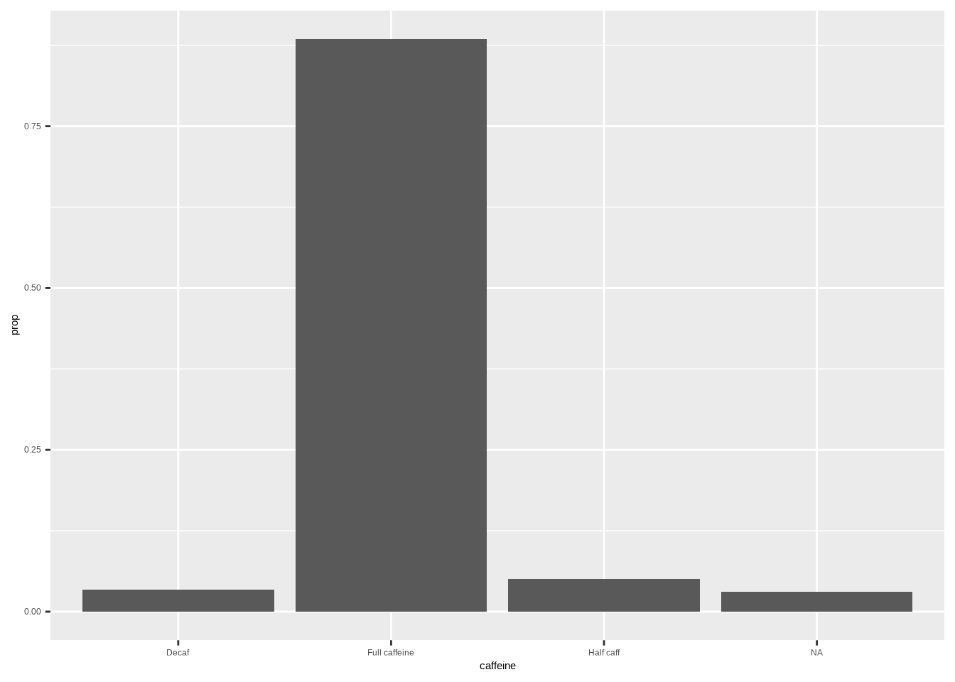
Note
Tip: Add labels/theme as needed: labs(x = "", y = "Proportion") + theme_minimal()
6 Two‑variable summaries (cross‑tabulation)
Suppose taste records whether participants like the taste of coffee.
6.1 Read the marginal distribution
cat_stats(coffee$taste)#> Continguency Table
#>
#> n prop
#> No 103 0.0289
#> Yes 3460 0.9711
#>
#> Number of Missing: 479
#> Proportion of Missing: 0.11850569025235
#> Row Variable: coffee$taste6.2 Cross‑tabulation (two‑way table)
- Rows: categories of one variable
- Columns: categories of the second variable
- Report counts or proportions by table, row, or column
Table proportions (each cell ÷ grand total):
cat_stats(coffee$caffeine, coffee$taste, prop = "table")#> Continguency Table
#>
#> No Yes Row Totals
#> Decaf "26 / 0.0073" "99 / 0.0279" "125 / 0.0352"
#> Full caffeine "66 / 0.0186" "3178 / 0.8957" "3244 / 0.9143"
#> Half caff "6 / 0.0017" "173 / 0.0488" "179 / 0.0505"
#> Col Totals "98 / 0.0276" "3450 / 0.9724" "Total: 3548"
#>
#> Cell Contents: n / tbl %
#> Col Totals Contents: n / row %
#> Row Totals Contents: n / col %
#> Column Variable: coffee$taste
#> Row Variable: coffee$caffeineRow proportions (each cell ÷ its row total):
cat_stats(coffee$caffeine, coffee$taste, prop = "row")#> Continguency Table
#>
#> No Yes Row Totals
#> Decaf "26 / 0.208" "99 / 0.792" "125 / 0.0352"
#> Full caffeine "66 / 0.0203" "3178 / 0.9797" "3244 / 0.9143"
#> Half caff "6 / 0.0335" "173 / 0.9665" "179 / 0.0505"
#> Col Totals "98 / 0.0276" "3450 / 0.9724" "Total: 3548"
#>
#> Cell Contents: n / row %
#> Col Totals Contents: n / row %
#> Row Totals Contents: n / col %
#> Column Variable: coffee$taste
#> Row Variable: coffee$caffeineColumn proportions (each cell ÷ its column total):
cat_stats(coffee$caffeine, coffee$taste, prop = "col")#> Continguency Table
#>
#> No Yes Row Totals
#> Decaf "26 / 0.2653" "99 / 0.0287" "125 / 0.0352"
#> Full caffeine "66 / 0.6735" "3178 / 0.9212" "3244 / 0.9143"
#> Half caff "6 / 0.0612" "173 / 0.0501" "179 / 0.0505"
#> Col Totals "98 / 0.0276" "3450 / 0.9724" "Total: 3548"
#>
#> Cell Contents: n / col %
#> Col Totals Contents: n / row %
#> Row Totals Contents: n / col %
#> Column Variable: coffee$taste
#> Row Variable: coffee$caffeine7 Stacked bar plots
Template:
ggplot(DATA, aes(x = VAR1, fill = VAR2)) +
  geom_bar()
Example (stacked counts):
ggplot(coffee, aes(x = caffeine, fill = taste)) +
  geom_bar()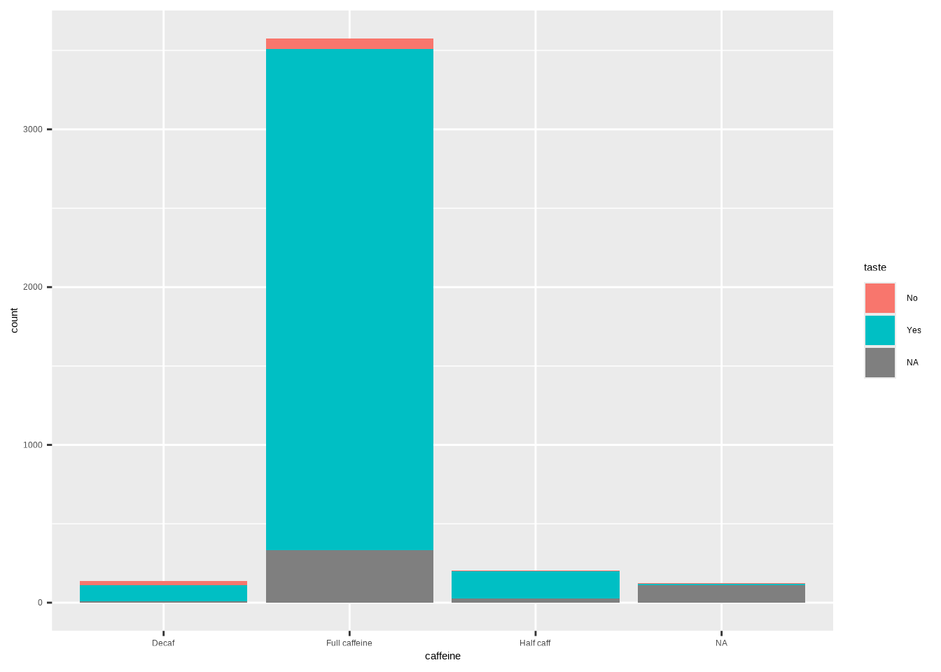
Example (horizontal):
ggplot(coffee, aes(y = caffeine, fill = taste)) +
  geom_bar()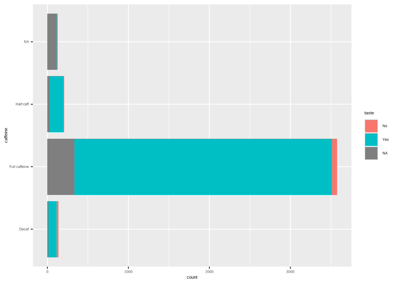
Template (stacked proportions):
ggplot(DATA, aes(x = VAR1, fill = VAR2)) +
  geom_bar(position = "fill") +
  labs(y = "Proportion")
8 Pie charts (use sparingly)
Note: Pie charts can be harder to compare precisely than bars. If you use them, label clearly.
Template:
df_pie <- cat_stats(DATA$VAR, tbl_df = TRUE)$table
ggplot(df_pie, aes(cat = Category, val = n, fill = Category)) +
  geom_pie()
Example:
coffee_pie <- cat_stats(coffee$caffeine, tbl_df = TRUE)$table
ggplot(coffee_pie, aes(cat = Category, val = n, fill = Category)) +
  geom_pie()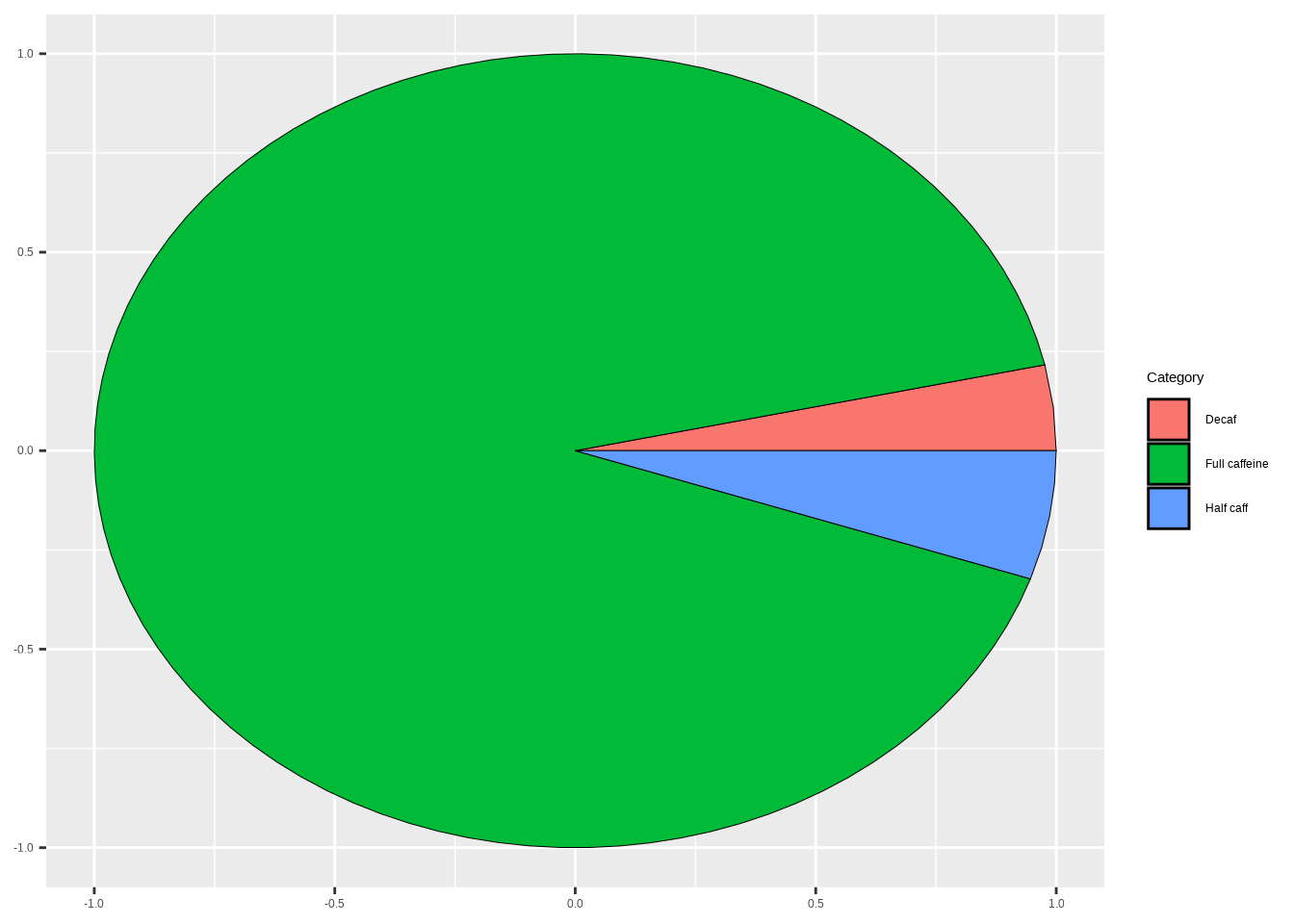
9 Mosaic plots
A mosaic plot shows a two‑way table with rectangle areas proportional to counts.
Template:
ggplot(DATA) +
  geom_mosaic(aes(x = product(VAR1, VAR2), fill = VAR2))
Example:
ggplot(coffee) +
  geom_mosaic(aes(x = product(caffeine, taste), fill = taste)) +
  labs(x = "caffeine × taste", y = "")
#> Warning: The `scale_name` argument of `continuous_scale()` is deprecated as of ggplot2
#> 3.5.0.#> Warning: The `trans` argument of `continuous_scale()` is deprecated as of ggplot2 3.5.0.
#> ℹ Please use the `transform` argument instead.#> Warning: `unite_()` was deprecated in tidyr 1.2.0.
#> ℹ Please use `unite()` instead.
#> ℹ The deprecated feature was likely used in the ggmosaic package.
#> Please report the issue at <https://github.com/haleyjeppson/ggmosaic>.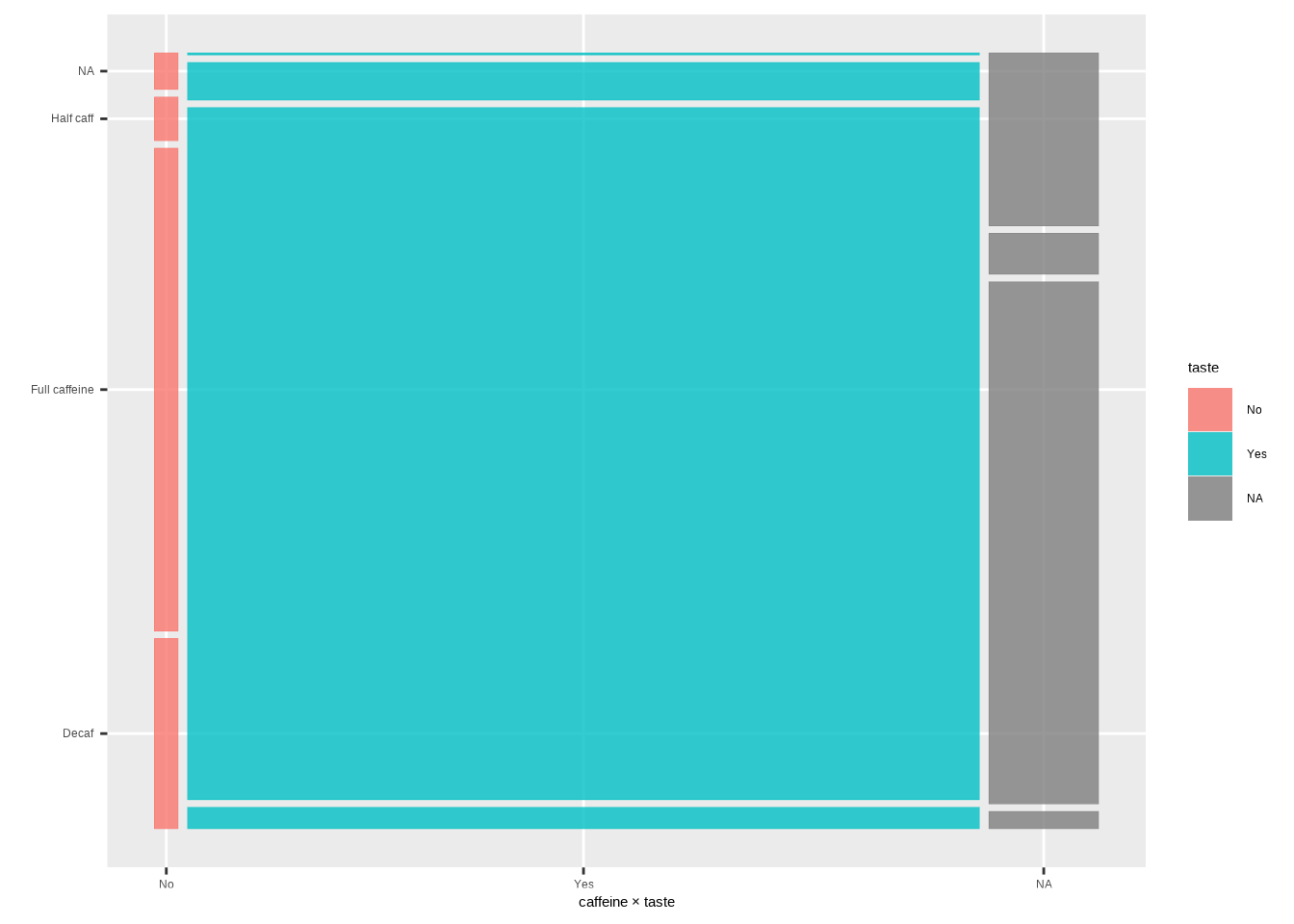
10 Waffle charts
A waffle chart is a 10×10‑style grid where each square often represents 1%.
Template:
waffle_df <- cat_stats(DATA$VAR, tbl_df = TRUE)$table
ggplot(waffle_df, aes(fill = Category, values = n)) +
  geom_waffle(make_proportional = TRUE)
Example:
coffee_waffle <- cat_stats(coffee$caffeine, tbl_df = TRUE)$table
ggplot(coffee_waffle, aes(fill = Category, values = n)) +
  geom_waffle(make_proportional = TRUE) +
  labs(x = NULL, y = NULL)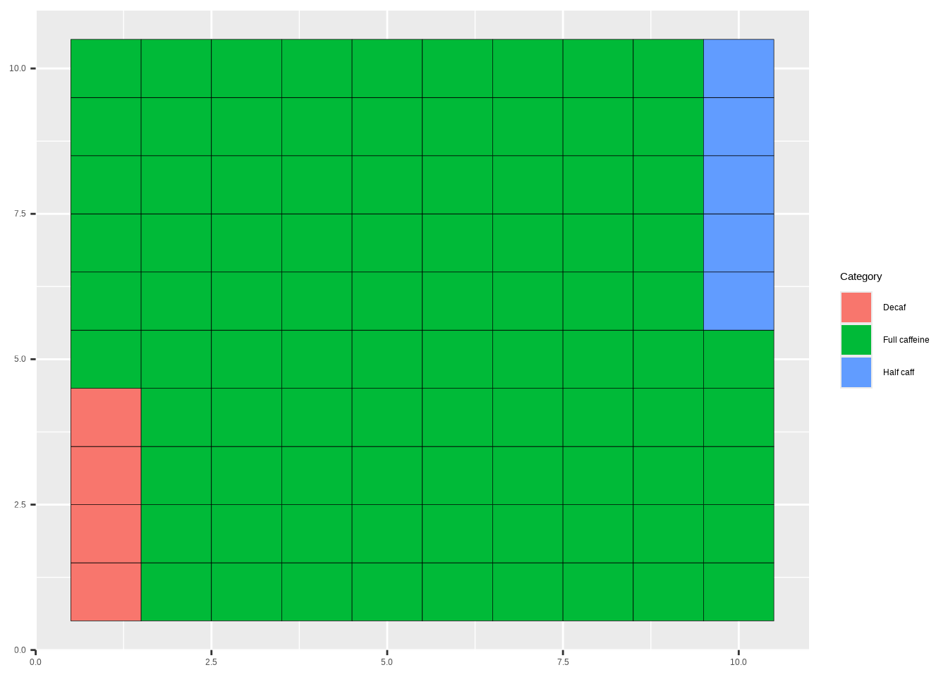
11 Appendix: minimal templates (copy‑paste)
Each template below has placeholders in ALL CAPS (e.g., DATA, VAR, VAR1, VAR2). Replace them with your own dataset name and variable names.
Note
How to customize placeholders: - DATA → the name of your dataset (e.g., coffee). - VAR → a single categorical variable (e.g., caffeine). - VAR1, VAR2 → two categorical variables for cross‑tabulations (e.g., caffeine, taste).
# Frequency table
cat_stats(DATA$VAR)
# Proportions only
cat_stats(DATA$VAR, prop_only = TRUE)# Bar: frequency
ggplot(DATA, aes(x = VAR)) +
geom_bar()# Bar: proportion
ggplot(DATA, aes(x = VAR, y = after_stat(prop), group = 1)) +
geom_bar()# Crosstab counts
cat_stats(DATA$VAR1, DATA$VAR2)# Crosstab proportions
cat_stats(DATA$VAR1, DATA$VAR2, prop = "table")
cat_stats(DATA$VAR1, DATA$VAR2, prop = "row")
cat_stats(DATA$VAR1, DATA$VAR2, prop = "col")# Stacked bar (counts)
ggplot(DATA, aes(x = VAR1, fill = VAR2)) + geom_bar()# Stacked bar (proportions)
ggplot(DATA, aes(x = VAR1, fill = VAR2)) +
geom_bar(position = "fill") + labs(y = "Proportion")# Pie
df_pie <- cat_stats(DATA$VAR, tbl_df = TRUE)$table
ggplot(df_pie, aes(cat = Category, val = n, fill = Category)) +
geom_pie()# Mosaic
ggplot(DATA) +
geom_mosaic(aes(x = product(VAR1, VAR2), fill = VAR2))# Waffle
wdf <- cat_stats(DATA$VAR, tbl_df = TRUE)$table
ggplot(wdf, aes(fill = Category, values = n)) +
geom_waffle(make_proportional = TRUE)