Not Dead… Yet!
An Introduction to Survival Analysis
Interval Censoring
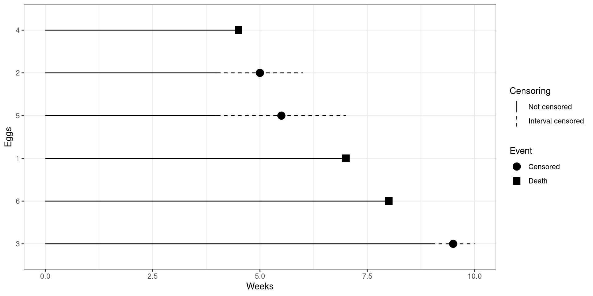
library(ggplot2)
dat <- structure(list(ID = 1:6,
                      eventA = c(0L, 1L, 1L, 0L, 1L, 0L),
                      eventB = c(1L, 0L, 0L, 1L, 0L, 1L),
                      t1 = c(7, 4, 9, 4.5, 4, 8),
                      t2 = c(7, 6, 10, 4.5, 7, 8),
                      censored = c(0, 1, 1, 0, 1, 0)),
                 .Names = c("ID", "eventA", "eventB", "t1", "t2", "censored"),
                 class = "data.frame", row.names = c(NA, -6L))

dat$event <- with(dat, ifelse(eventA, "Censored", "Death"))

dat$id.ordered <- factor(x = dat$ID, levels = order(dat$t2, decreasing = T))

ggplot(dat, aes(x = id.ordered)) +
    geom_linerange(aes(ymin = 0, ymax = t1)) +
    geom_linerange(aes(ymin = t1, ymax = t2,
                       linetype = as.factor(censored))) +
    geom_point(aes(y = ifelse(censored,
                              t1 + (t2 - t1) / 2, t2),
                   shape = event), size = 4) +
    coord_flip() +
    scale_linetype_manual(name = "Censoring", values = c(1, 2),
        labels = c("Not censored", "Interval censored")) +
    scale_shape_manual(name = "Event", values = c(19, 15)) +
    # ggtitle("Interval Censoring") +
    xlab("Eggs") +  ylab("Weeks") +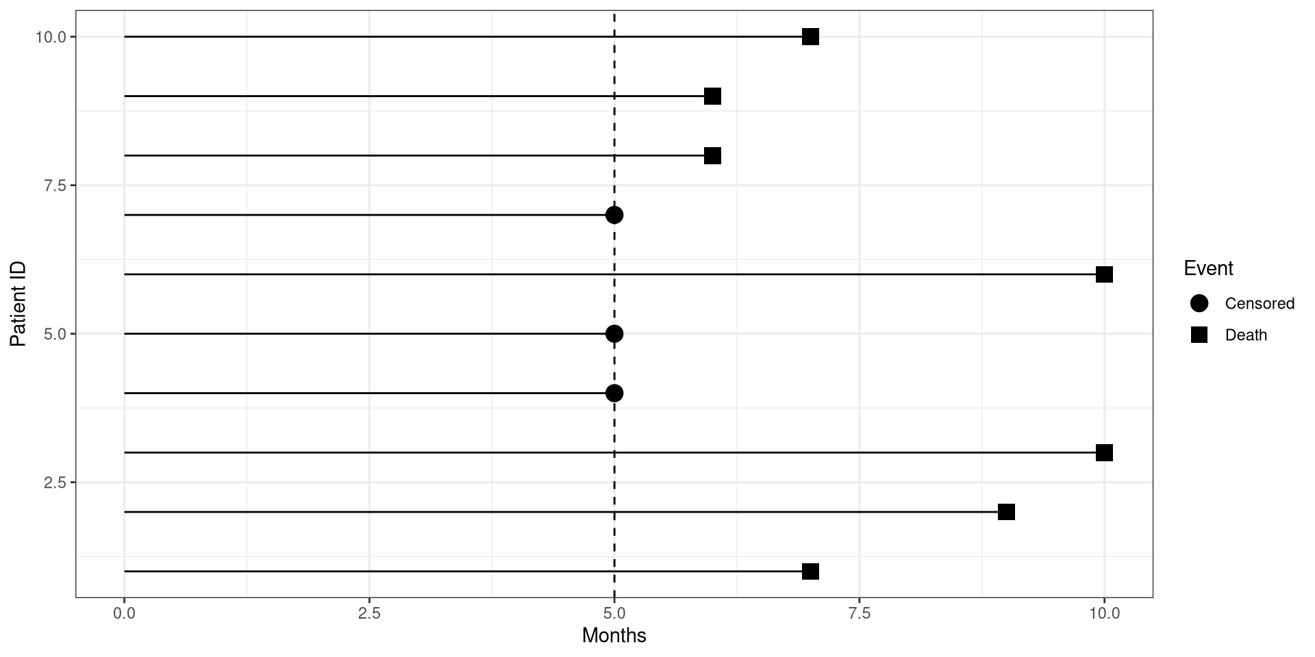
theme_bw()Right Censoring
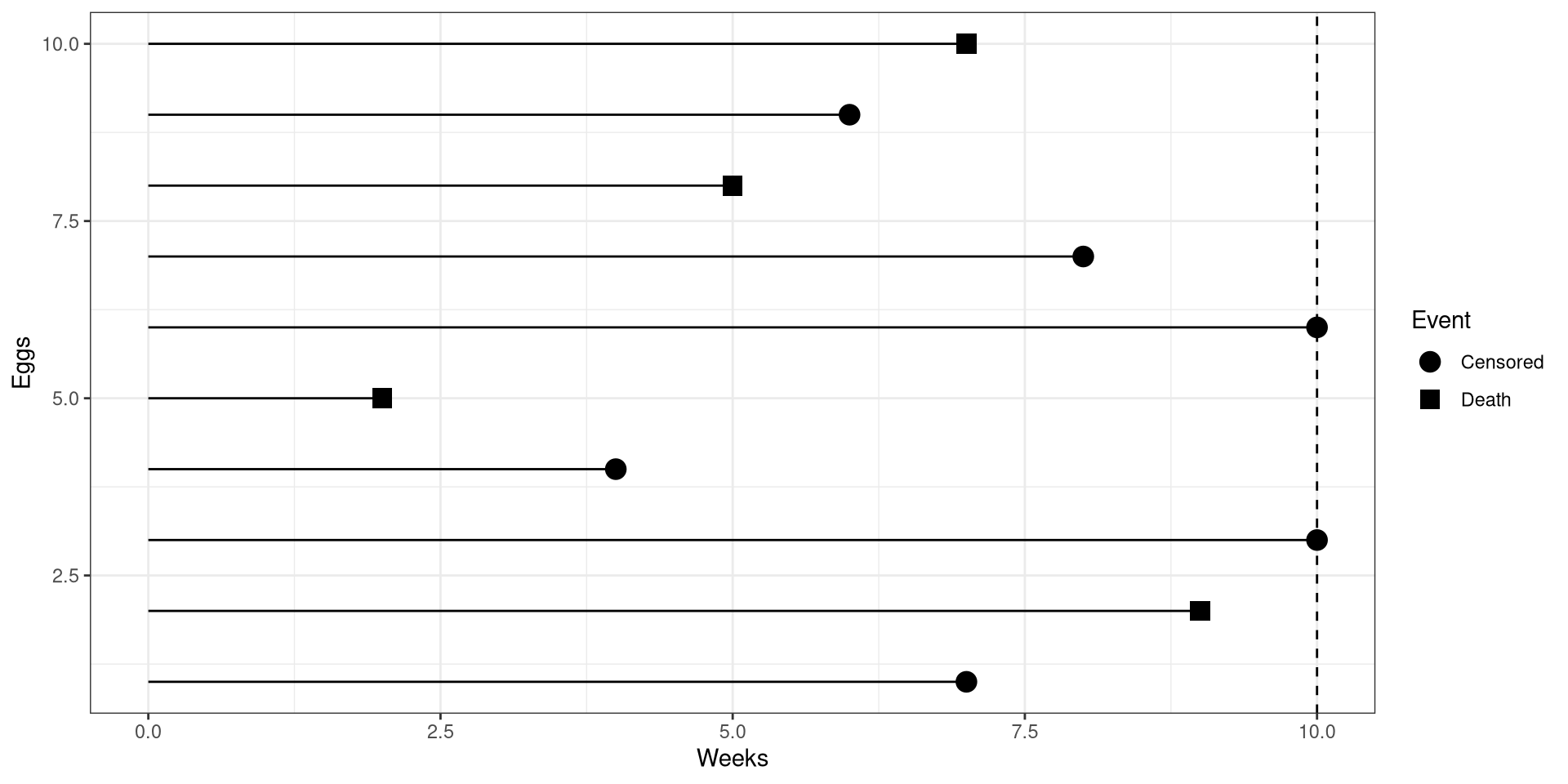
library(ggplot2)
dat <- data.frame(ID = 1:10,
                  t1 = c(7, 9, 10, 4, 2, 10, 8, 5, 6, 7) ,
                  censored = c(0, 1, 0, 0, 1, 0, 0, 1, 0, 1))
ggplot(dat, aes(x = ID, y = t1,
                shape = ifelse(censored, "Death", "Censored"))) +
    geom_point(size = 4) +
    geom_linerange(aes(ymin = 0, ymax = t1)) +
    geom_hline(yintercept = 10, lty = 2) +
    coord_flip() +
    scale_shape_manual(name = "Event", values = c(19, 15)) +
    # ggtitle("Right Censoring") +
    xlab("Patient ID") +  ylab("Months") +
theme_bw()Survival Curve
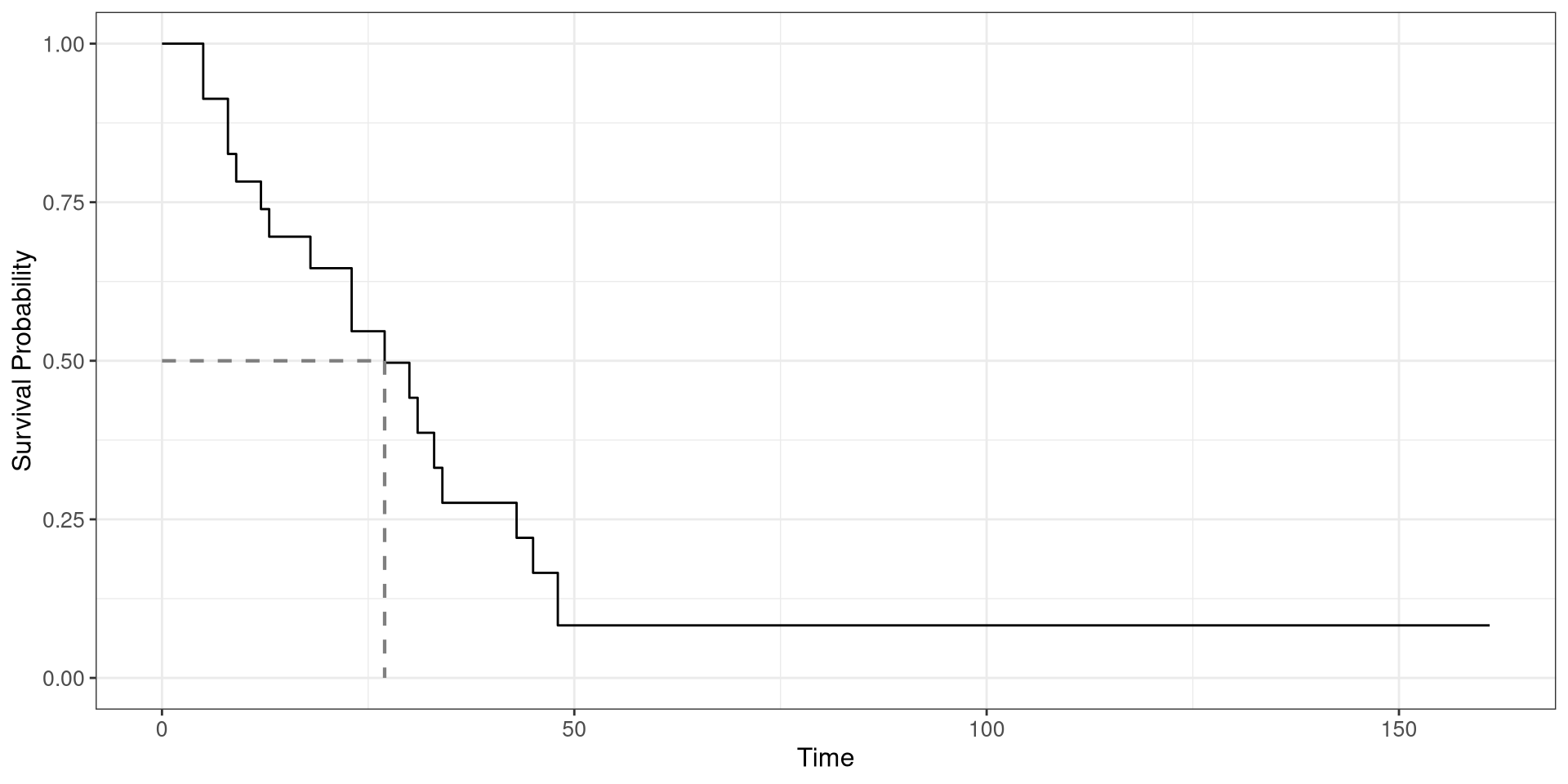
Colon Survival Curve
- Fit a survival curve using
df_colonfrom theggsurvfitpackage. time: time-to-deathstatus: censoring status- Plot the survival curve and add a line indicating the 50th percentile
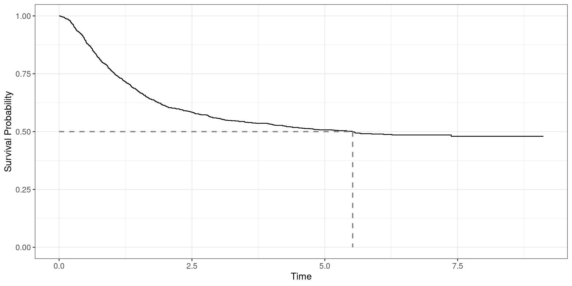
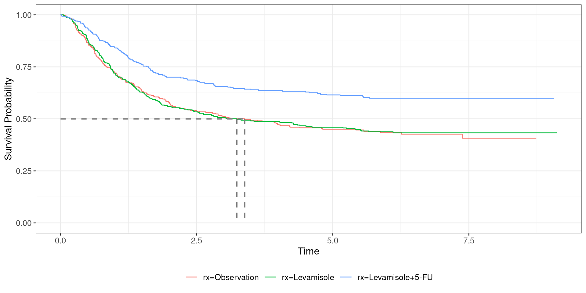
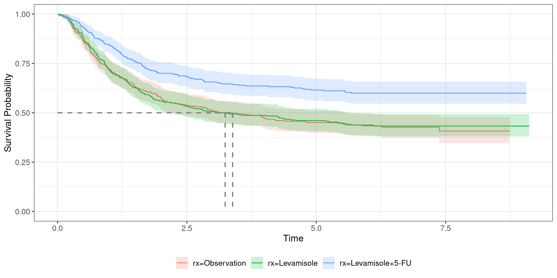
Colon Survival Curve
- Fit a survival curve using
df_colon, stratified by treatment regimen time: time-to-deathstatus: censoring statusrx: treatment regimen- Plot the curvival curve and add a line indicating the 50th percentile