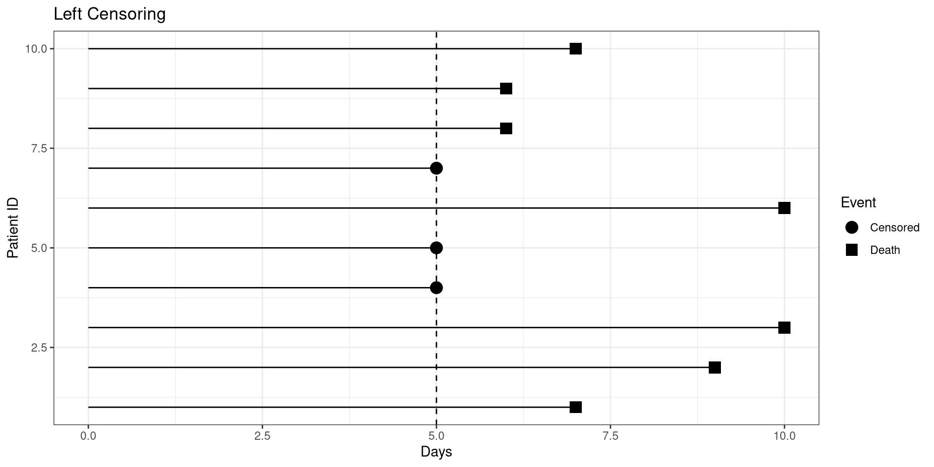
library(ggplot2)
dat <- data.frame(ID = 1:10,
                  t1 = c(7, 9, 10, 5, 5, 10, 5, 6, 6, 7) ,
                  censored = c(1, 1, 1, 0, 0, 1, 0, 1, 1, 1))
ggplot(dat, aes(x = ID, y = t1, shape = ifelse(censored, "Death", "Censored"))) + geom_point(size = 4) +
    geom_linerange(aes(ymin = 0, ymax = t1)) +
    geom_hline(yintercept = 5, lty = 2) +
    coord_flip() +
    scale_shape_manual(name = "Event", values = c(19, 15)) +
    ggtitle("Left Censoring") +
    xlab("Patient ID") +  ylab("Days") +
theme_bw()Survival Analysis:
The Life and Death of Statistics
Left Censoring
Interval Censoring
library(ggplot2)
dat <- structure(list(ID = 1:5, eventA = c(0L, 1L, 1L, 0L, 1L),
    eventB = c(1L, 0L, 0L, 1L, 0L), t1 = c(7, 5, 10, 4.5, 2), t2 = c(7, 5, 10, 4.5,
    8), censored = c(0, 0, 0, 0, 1)), .Names = c("ID", "eventA",
    "eventB", "t1", "t2", "censored"), class = "data.frame", row.names = c(NA, -5L))

dat$event <- with(dat, ifelse(eventA, "Censored", "Death"))

dat$id.ordered <- factor(x = dat$ID, levels = order(dat$t2, decreasing = T))

ggplot(dat, aes(x = id.ordered)) +
    geom_linerange(aes(ymin = 0, ymax = t1)) +
    geom_linerange(aes(ymin = t1, ymax = t2,
                       linetype = as.factor(censored))) +
    geom_point(aes(y = ifelse(censored,
                              t1 + (t2 - t1) / 2, t2),
                   shape = event), size = 4) +
    coord_flip() +
    scale_linetype_manual(name = "Censoring", values = c(1, 2),
        labels = c("Not censored", "Interval censored")) +
    scale_shape_manual(name = "Event", values = c(19, 15)) +
    ggtitle("Interval Censoring") +
    xlab("Patient ID") +  ylab("Days") +
    theme_bw()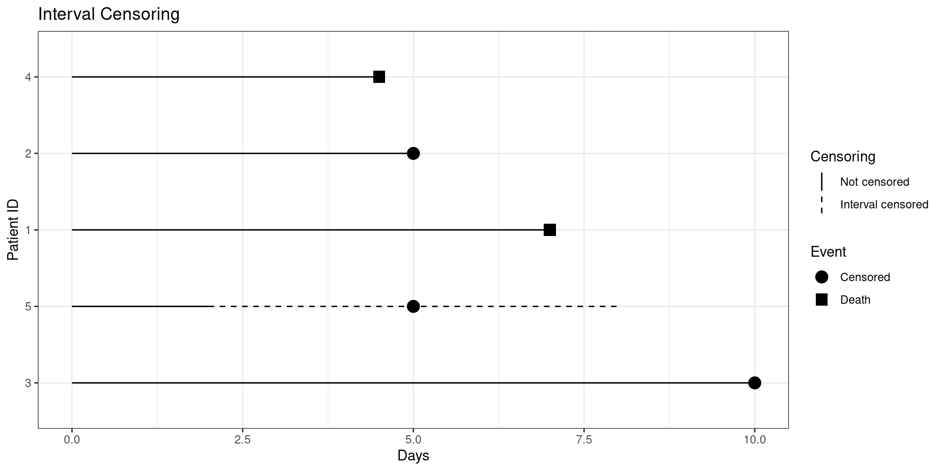
Right Censoring
library(ggplot2)
dat <- data.frame(ID = 1:10,
                  t1 = c(7, 9, 10, 4, 2, 10, 8, 5, 6, 7) ,
                  censored = c(0, 1, 0, 0, 1, 0, 0, 1, 0, 1))
ggplot(dat, aes(x = ID, y = t1,
                shape = ifelse(censored, "Death", "Censored"))) +
    geom_point(size = 4) +
    geom_linerange(aes(ymin = 0, ymax = t1)) +
    geom_hline(yintercept = 10, lty = 2) +
    coord_flip() +
    scale_shape_manual(name = "Event", values = c(19, 15)) +
    ggtitle("Right Censoring") +
    xlab("Patient ID") +  ylab("Days") +
    theme_bw()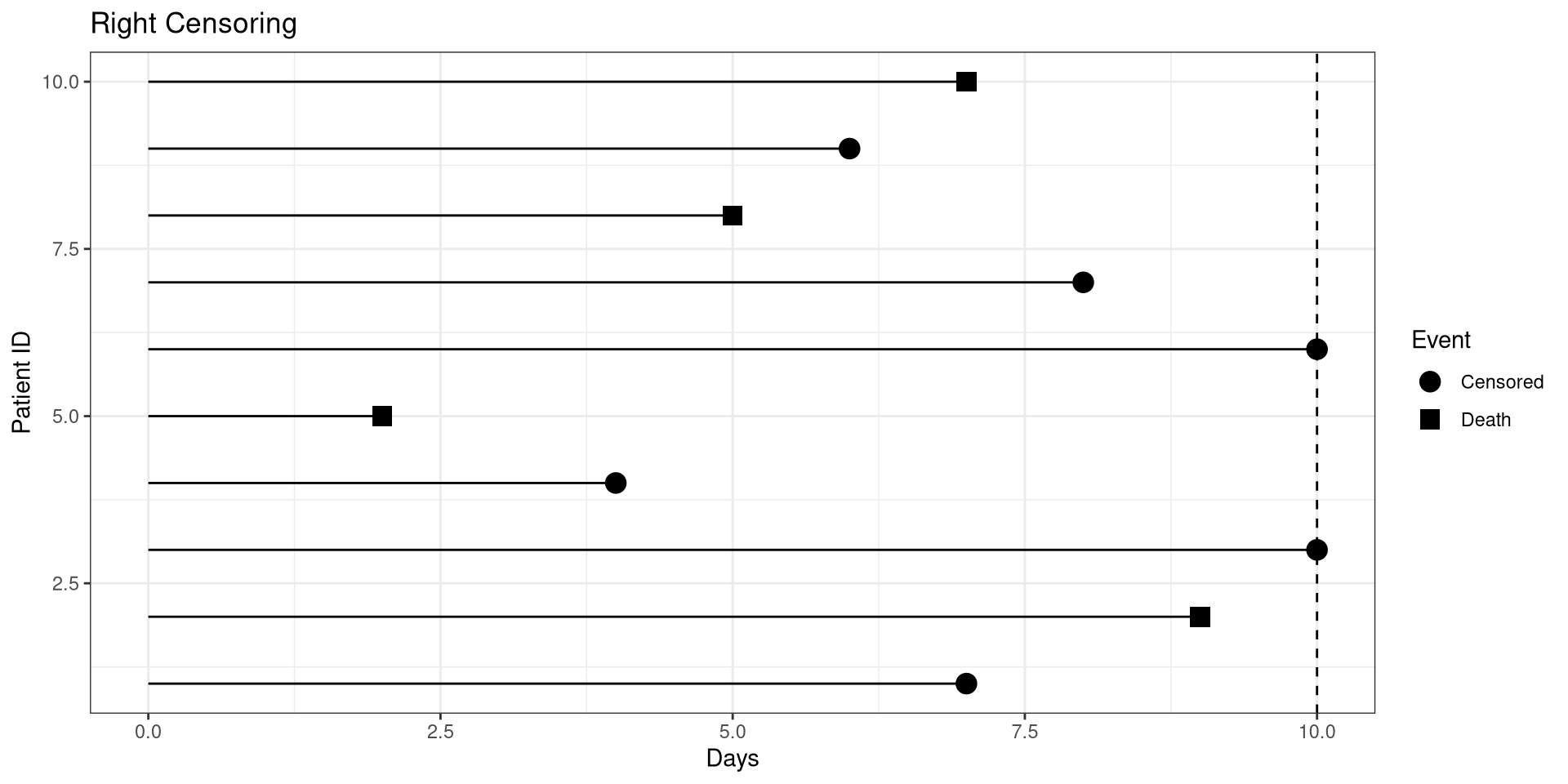
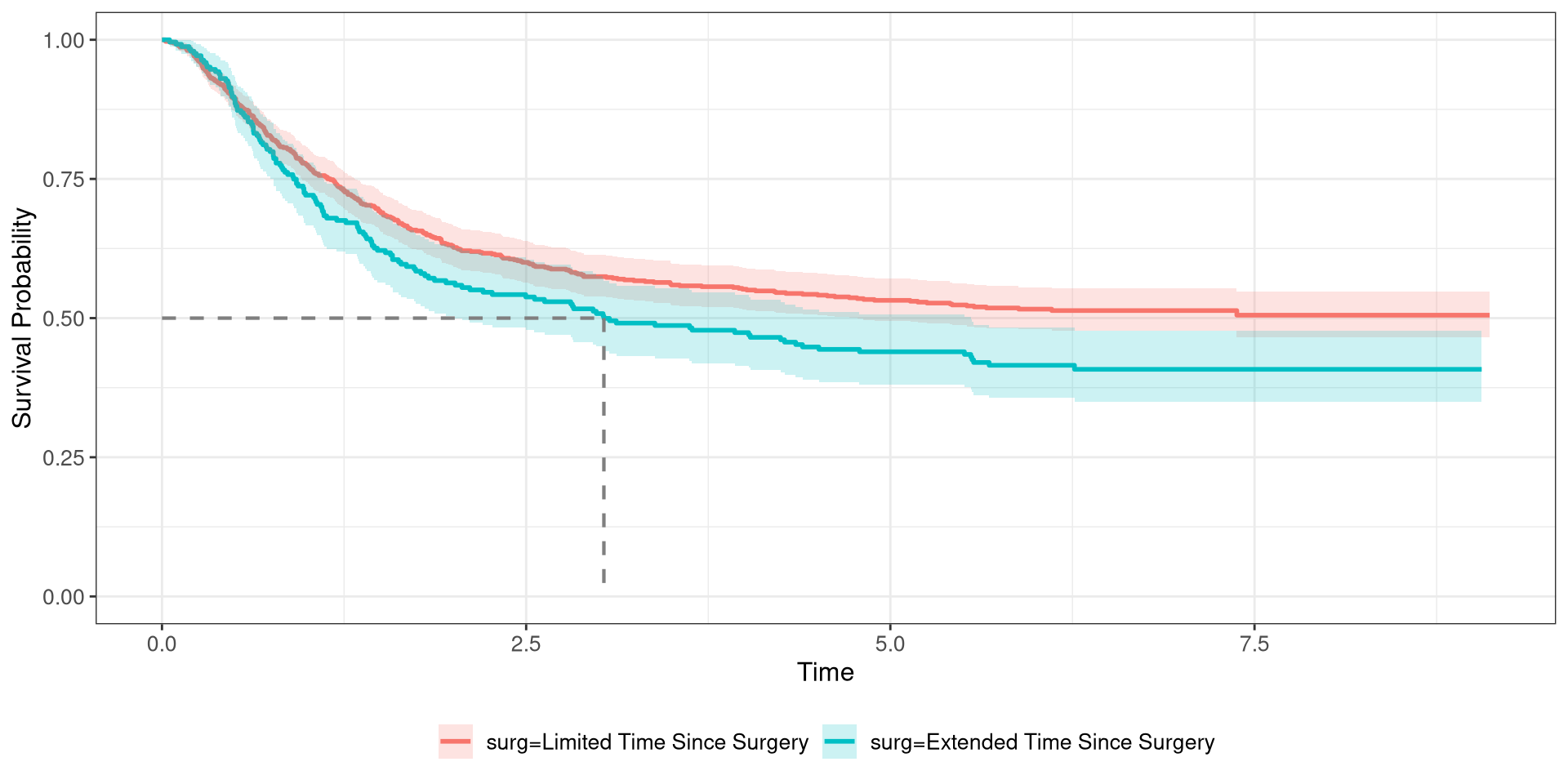
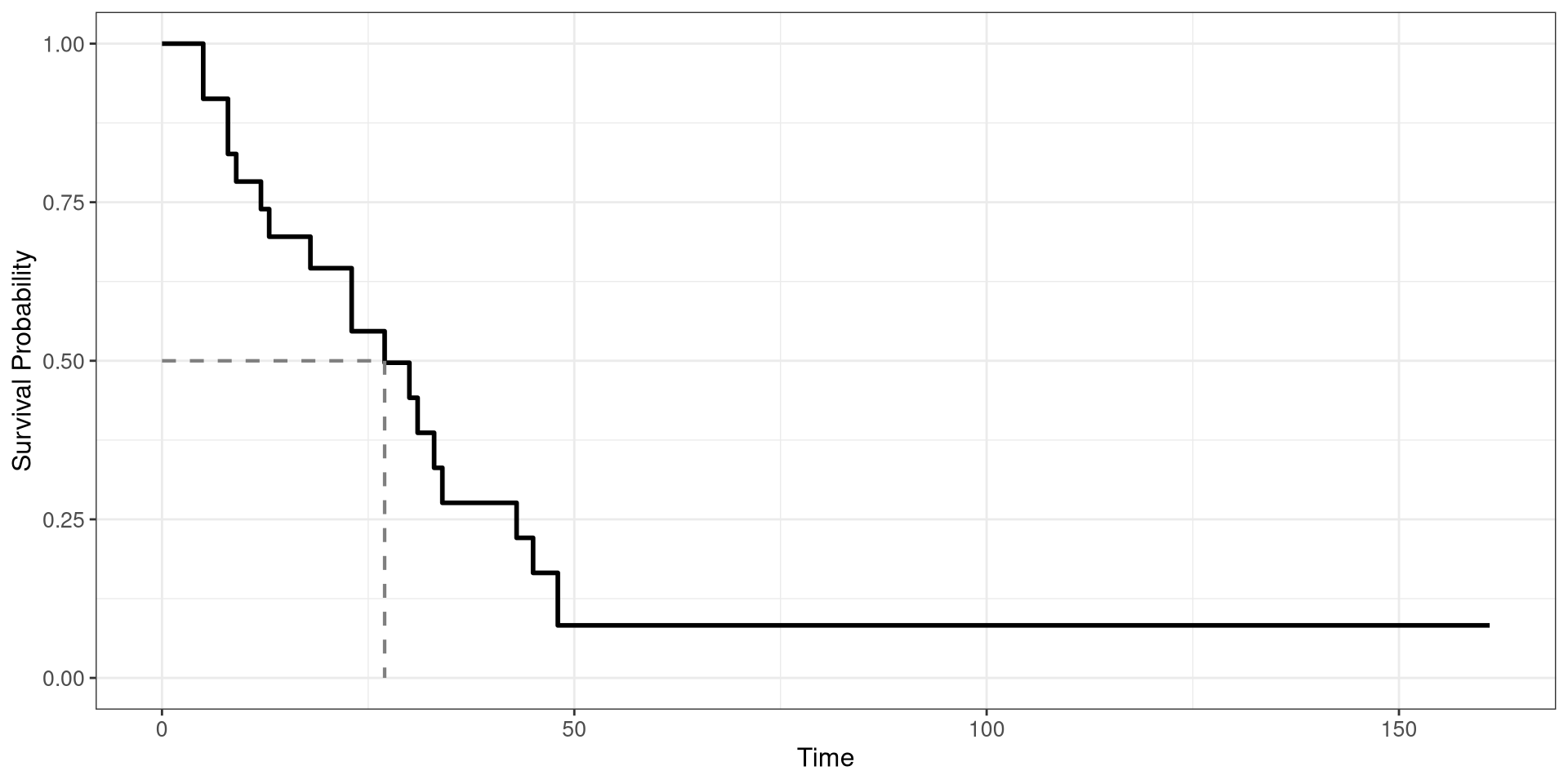
Survival Curve
Colon Survival Curve
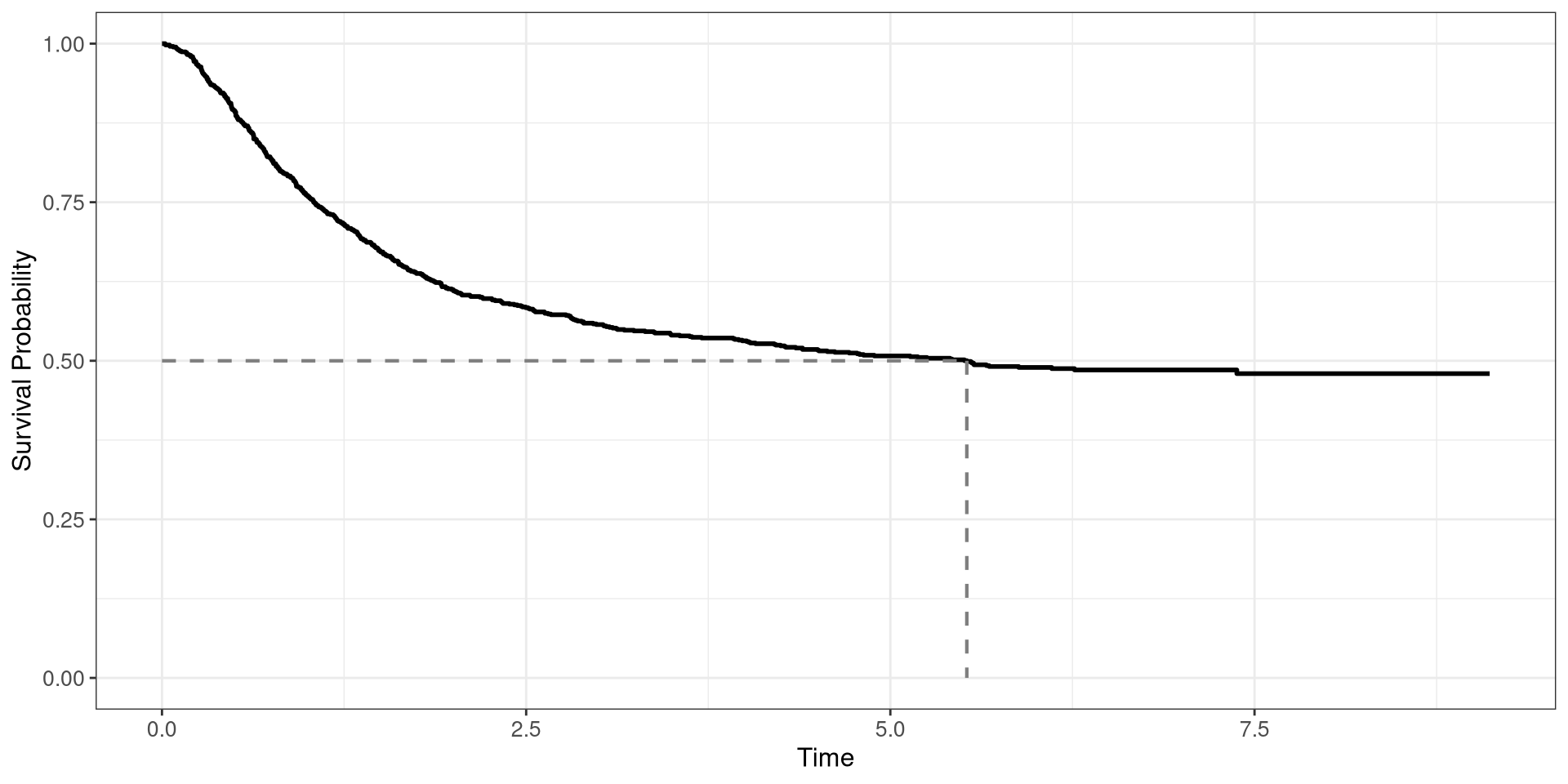
Colon Survival Curve
Colon Survival Curve
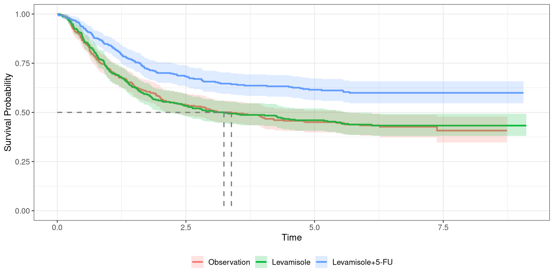
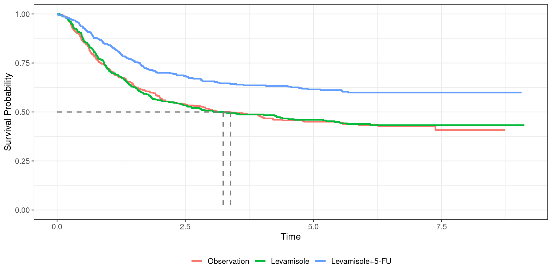
Fitting a Survival Curve
1library(magrittr)
2library(survival)
3library(ggsurvfit)
4df_colon %$% survfit(Surv(time, status) ~ surg)  %>%
5      ggsurvfit(linewidth = 1) +
6      add_confidence_interval() +
7 add_quantile(y_value = 0.5, color = "gray50", linewidth = 0.75)- 1
- Pipe package
- 2
- Survival functions package
- 3
- Plots survival curves package
- 4
- Applies the Kaplan-Meier Function
- 5
- Plots Survival Curve
- 6
- Adds Confidence Intervals
- 7
- Determines Median Survival Time