Code
library(ggplot2)library(ggplot2)When collecting a random sample, it is believed that the data being collected comes from a probability distribution denoted as \(F(\boldsymbol \theta)\), where \(\boldsymbol \theta = (\theta_1, \theta_2, \ldots, \theta_p)^{\mathrm T}\) is a vector or parameters that describe the distribution. It is assumed that the random sample is a collection of random variables, denoted as \(X_1, \cdots, X_n\), that are considered iid (identical and independently distributed1). Using this random sample, one infer the value of the parameters \(\boldsymbol \theta\) by functions (statistics) on the random sample.
A statistical estimator is said to be a function designed to provide a point estimate, or interval estimate, of an unknown parameter in \(\boldsymbol \theta\). Common statistical estimators can be the mean, \(\bar X = \frac{1}{n}\sum^n_{i=1} X_i\), or standard deviation, \(S^2 = \frac{1}{n-1}\sum^{n}_{i=1}(X_i - \bar X)^2\). Other estimators can be obtained by applying a procedure such as the maximum likelihood estimation, method of moments or a Bayes Estimator.
A sampling distribution can be thought as the distribution of an estimator (statistic). The reason is because the estimator is a function of random variables; therefore, the estimator itself is also a random variable. This means that the estimator will vary based on what was randomly drawn for the sample. For example, \(\bar X = \frac{1}{n}\sum^n_{i=1}X_i\) will have a distribution depending on the distribution that generated \(X_1, \ldots, X_n\).
Assume that \(X_1, \ldots, X_{25}\overset{iid}{\sim}N(8, 3)\), normal distribution with mean 8 and variance 3. Depending on the sample, the value of \(\bar X\) will change due to the randomness being generated. Therefore, a different sample will yield a different value of \(\bar X\). The R code below will demonstrate the potential distribution \(\bar X\) by simulating numerous samples from distribution above and generating the histogram of \(\bar X\).
To simulate a random sample of 25 that follows a normal distribution, we can use the rnorm function. Afterwards, we will compute the mean of the sample.
x1 <- rnorm(25, 8, sqrt(3))
mean(x1)
#> [1] 8.136938Notice that the value is close to 8. Generate (run the code below) multiple samples and see what mean are values are being produced:
Now to visualize see the distribution of \(\bar X\), we will simulate 10,000 samples, compute the mean of each sample, and construct the a histogram of the computed means.
# Generate 10,000 samples of size 25
x_samples <- replicate(10000, rnorm(25, 8, sqrt(3)))
# Obtain the mean for all the samples
x_means <- colMeans(x_samples)
# Plot a histogram of the sample means
data.frame(xbar = x_means) |>
  ggplot(aes(xbar)) +
  geom_histogram() +
  theme_bw()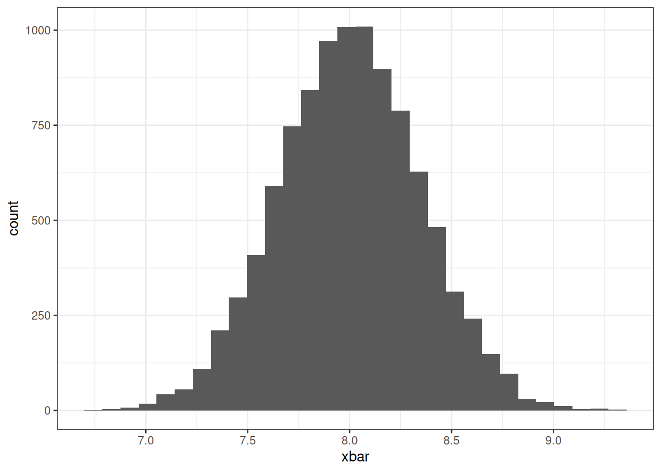
Notice that the values of \(\bar X\) are bell shaped centered around the value 8. This makes us think that the sampling distribution for \(\bar X\) may follow a normal distribution. In fact, if a random sample is said to be generated from a normal distribution, then the distribution will also be normally distributed. For this example, the distribution of \(\bar X\) is \(N(8, 3/25)\). We can plot the probability density function on the histogram and they will closely align.
# Plotting the histogram of the sample means
# And imposing the density function of a normal distribution

data.frame(xbar = x_means, y = dnorm(x_means, 8, sqrt(3/25))) |>
  ggplot(aes(xbar, y = after_stat(density))) +
  geom_histogram() +
  geom_line(aes(xbar, y), col = "red", lwd = 1) +
  theme_bw()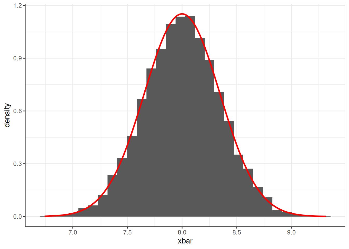
The central limit theorem is the framework for several of hypothesis tests that are based on probability models.
If random variables \(X_1, X_2, \cdots, X_n\) are independent come from the same distribution (\(iid\)), \(E(X_i) = \mu <\infty\) (finite), \(Var(X_i) = \sigma^2<\infty\) (finite), then
\[ \frac{\bar X - \mu}{\sigma/\sqrt n} \overset{\circ}{\sim} N(0,1) \]
as \(n\rightarrow \infty\), which implies:
\[ \bar X \overset{\circ}{\sim} N(\mu, \sigma^2/n) \]
The central limit theorem allows us to assume the distribution of \(\bar X\) regardless of the distribution of the sample \(X_1, X_2, \cdots, X_n\). The only condition is that the expected value and variance exist.
Assume that \(X_1, \ldots, X_{n}\overset{iid}{\sim}\chi^2(4)\), Chi-Square distribution with 4 degrees of freedom. According to the central limit theorem, as \(n\rightarrow \infty\), the distribution for \(\bar X\) will approximately be normal with a mean of \(4\) and variance \(8/n\).
Run the following examples to show how the distribution begins to follow a normal distribution (red line) as \(n\) increases 15, 30, 50, 100, 1000. Change the number on line 3 to see how the distribtion changes.
Assume that \(X_1, \ldots, X_{n}\overset{iid}{\sim}Pois(3.2)\), Poisson distribution with a rate of 3.2. According to the central limit theorem, as \(n\rightarrow \infty\), the distribution for \(\bar X\) will approximately be normal with a mean of \(3.2\) and variance \(3.2/n\).
Run the following examples to show how the distribution begins to follow a normal distribution (red line) as \(n\) increases 15, 30, 50, 100, 1000. Change the number on line 3 to see how the distribtion changes.